Keras_cv_attention_models
- 警告:目前与
keras 3.x 不兼容。如果使用 tensorflow>=2.16.0,需要手动安装 pip install tf-keras~=$(pip show tensorflow | awk -F ': ' '/Version/{print $2}')。导入时,请先于 Tensorflow 导入本包,或设置 export TF_USE_LEGACY_KERAS=1。
- 不建议直接从 h5 文件下载并加载模型,最好通过构建模型后再加载权重,例如
import kecam; mm = kecam.models.LCNet050()。
- 用于 TF 的 coco_train_script.py 仍在测试中……
通用用法
基础
- 默认导入 在 README 中使用时不会特别说明。
import os
import sys
import tensorflow as tf
import numpy as np
import pandas as pd
import matplotlib.pyplot as plt
from tensorflow import keras
- 以 pip 包形式安装。
kecam 是本包的简称。注意:pip 包 kecam 不设定任何后端要求,请确保事先已安装 Tensorflow 或 PyTorch。如需使用 PyTorch 后端,请参阅 Keras PyTorch 后端。pip install -U kecam
# 或
pip install -U keras-cv-attention-models
# 或
pip install -U git+https://github.com/leondgarse/keras_cv_attention_models
具体用法请参考各子目录。
- 基础模型预测
from keras_cv_attention_models import volo
mm = volo.VOLO_d1(pretrained="imagenet")

""" 运行预测 """
import tensorflow as tf
from tensorflow import keras
from keras_cv_attention_models.test_images import cat
img = cat()
imm = keras.applications.imagenet_utils.preprocess_input(img, mode='torch')
pred = mm(tf.expand_dims(tf.image.resize(imm, mm.input_shape[1:3]), 0)).numpy()
pred = tf.nn.softmax(pred).numpy()  # 如果分类器激活函数不是 softmax
print(keras.applications.imagenet_utils.decode_predictions(pred)[0])
# [('n02124075', '埃及猫', 0.99664897),
#  ('n02123045', '虎斑猫', 0.0007249644),
#  ('n02123159', '虎猫', 0.00020345),
#  ('n02127052', '猞猁', 5.4973923e-05),
#  ('n02123597', '暹罗猫', 2.675306e-05)]
或者直接使用模型预设的 preprocess_input 和 decode_predictionsfrom keras_cv_attention_models import coatnet
mm = coatnet.CoAtNet0()
from keras_cv_attention_models.test_images import cat
preds = mm(mm.preprocess_input(cat()))
print(mm.decode_predictions(preds))
# [[('n02124075', '埃及猫', 0.9999875), ('n02123045', '虎斑猫', 5.194884e-06), ...]]
预设的 preprocess_input 和 decode_predictions 也兼容 PyTorch 后端。os.environ['KECAM_BACKEND'] = 'torch'
from keras_cv_attention_models import caformer
mm = caformer.CAFormerS18()
# >>>> 使用 PyTorch 后端
# >>>> 对齐输入形状:[3, 224, 224]
# >>>> 从 ~/.keras/models/caformer_s18_224_imagenet.h5 加载预训练权重
from keras_cv_attention_models.test_images import cat
preds = mm(mm.preprocess_input(cat()))
print(preds.shape)
# torch.Size([1, 1000])
print(mm.decode_predictions(preds))
# [[('n02124075', '埃及猫', 0.8817097), ('n02123045', '虎斑猫', 0.009335292), ...]]
```
- 设置
num_classes=0 以排除模型顶部的 GlobalAveragePooling2D + Dense 层。from keras_cv_attention_models import resnest
mm = resnest.ResNest50(num_classes=0)
print(mm.output_shape)
# (None, 7, 7, 2048)
- 如果
num_classes={自定义输出类别} 不是 1000 或 0,则会跳过加载头部的 Dense 层权重。这是因为使用了 model.load_weights(weight_file, by_name=True, skip_mismatch=True) 来加载权重。from keras_cv_attention_models import swin_transformer_v2
mm = swin_transformer_v2.SwinTransformerV2Tiny_window8(num_classes=64)
# >>>> 从 ~/.keras/models/swin_transformer_v2_tiny_window8_256_imagenet.h5 加载预训练权重
# WARNING:tensorflow:由于权重 predictions/kernel:0 的形状不匹配,跳过加载第 601 层(名为 predictions)的权重。该权重期望形状为 (768, 64),而保存的权重形状为 (768, 1000)。
# WARNING:tensorflow:由于权重 predictions/bias:0 的形状不匹配,跳过加载第 601 层(名为 predictions)的权重。该权重期望形状为 (64,),而保存的权重形状为 (1000,)。
- 可以通过设置
pretrained="xxx.h5" 重新加载自己的模型权重。与直接调用 model.load_weights 相比,这种方法在重新加载具有不同 input_shape 且权重形状不匹配的模型时更为优越。import os
from keras_cv_attention_models import coatnet
pretrained = os.path.expanduser('~/.keras/models/coatnet0_224_imagenet.h5')
mm = coatnet.CoAtNet1(input_shape=(384, 384, 3), pretrained=pretrained) # 没什么意义,只是为了展示用法
- 可以使用别名
kecam 代替 keras_cv_attention_models。它只是一个仅包含 from keras_cv_attention_models import * 的 __init__.py 文件。import kecam
mm = kecam.yolor.YOLOR_CSP()
imm = kecam.test_images.dog_cat()
preds = mm(mm.preprocess_input(imm))
bboxs, lables, confidences = mm.decode_predictions(preds)[0]
kecam.coco.show_image_with_bboxes(imm, bboxs, lables, confidences)
- 使用 TF 2.0 功能:FLOPs 计算 #32809 中的方法计算 FLOPs。对于 PyTorch 后端,需要安装
thop:pip install thop。from keras_cv_attention_models import coatnet, resnest, model_surgery
model_surgery.get_flops(coatnet.CoAtNet0())
# >>>> FLOPs: 4,221,908,559, GFLOPs: 4.2219G
model_surgery.get_flops(resnest.ResNest50())
# >>>> FLOPs: 5,378,399,992, GFLOPs: 5.3784G
- [已弃用]
tensorflow_addons 默认不会被导入。如果直接从 h5 文件中加载依赖于 GroupNormalization 的模型(如 MobileViTV2),则需要先手动导入 tensorflow_addons。import tensorflow_addons as tfa
model_path = os.path.expanduser('~/.keras/models/mobilevit_v2_050_256_imagenet.h5')
mm = keras.models.load_model(model_path)
- 将 TF 模型导出为 ONNX 格式。对于 TF 需要
tf2onnx:pip install onnx tf2onnx onnxsim onnxruntime。对于 PyTorch 后端,PyTorch 本身支持导出 ONNX 模型。from keras_cv_attention_models import volo, nat, model_surgery
mm = nat.DiNAT_Small(pretrained=True)
model_surgery.export_onnx(mm, fuse_conv_bn=True, batch_size=1, simplify=True)
# 导出的简化 ONNX:dinat_small.onnx
# 运行测试
from keras_cv_attention_models.imagenet import eval_func
aa = eval_func.ONNXModelInterf(mm.name + '.onnx')
inputs = np.random.uniform(size=[1, *mm.input_shape[1:]]).astype('float32')
print(f"{np.allclose(aa(inputs), mm(inputs), atol=1e-5) = }")
# np.allclose(aa(inputs), mm(inputs), atol=1e-5) = True
- 模型摘要
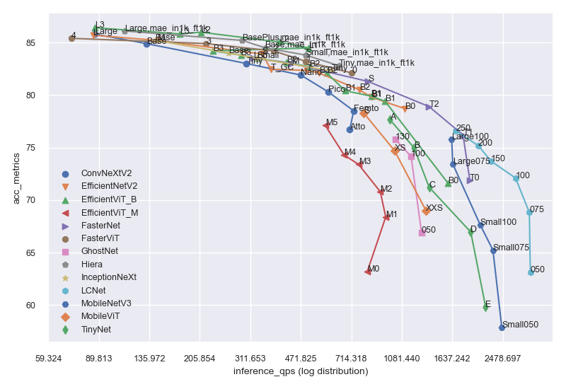
model_summary.csv 包含汇总的模型信息。
params 表示模型参数数量,单位为 Mflops 表示 FLOPs 数量,单位为 Ginput 表示模型输入形状acc_metrics 表示识别模型的 Imagenet Top1 Accuracy,检测模型的 COCO val APinference_qps 表示使用 batch_size=1 + trtexec 时的 T4 推理每秒查询数extra 表示是否有额外的训练信息。
from keras_cv_attention_models import plot_func
plot_series = [
    "efficientnetv2", 'tinynet', 'lcnet', 'mobilenetv3', 'fasternet', 'fastervit', 'ghostnet',
    'inceptionnext', 'efficientvit_b', 'mobilevit', 'convnextv2', 'efficientvit_m', 'hiera',
]
plot_func.plot_model_summary(
    plot_series, model_table="model_summary.csv", log_scale_x=True, allow_extras=['mae_in1k_ft1k']
)
- 代码格式 使用
line-length=160:find ./* -name "*.py" | grep -v __init__ | xargs -I {} black -l 160 {}
T4 推理
- 模型表格中的 T4 推理 数据是在
Tesla T4 上使用 trtexec 测试得到的,使用的环境为 CUDA=12.0.1-1, Driver=525.60.13。所有模型均使用 PyTorch 后端导出为 ONNX 格式,且仅使用 batch_size=1。注意:这些数据仅供参考,在不同的批量大小、基准测试工具、平台或实现方式下可能会有所不同。
- 所有结果均在 colab 的 trtexec.ipynb 中测试完成,因此任何人都可以复现。
os.environ["KECAM_BACKEND"] = "torch"

from keras_cv_attention_models import convnext, test_images, imagenet
# >>>> 使用 PyTorch 后端
mm = convnext.ConvNeXtTiny()
mm.export_onnx(simplify=True)
# 导出的 ONNX:convnext_tiny.onnx
# 正在运行 onnxsim.simplify...
# 导出的简化 ONNX:convnext_tiny.onnx

# ONNX 运行测试
tt = imagenet.eval_func.ONNXModelInterf('convnext_tiny.onnx')
print(mm.decode_predictions(tt(mm.preprocess_input(test_images.cat()))))
# [[('n02124075', '埃及猫', 0.880507), ('n02123045', '虎斑猫', 0.0047998047), ...]]

""" 运行 trtexec 基准测试 """
!trtexec --onnx=convnext_tiny.onnx --fp16 --allowGPUFallback --useSpinWait --useCudaGraph
层
- attention_layers 仅是一个
__init__.py 文件,它导入了模型架构中定义的核心层。例如来自 botnet 的 RelativePositionalEmbedding,来自 volo 的 outlook_attention,以及其他许多 Positional Embedding Layers / Attention Blocks。from keras_cv_attention_models import attention_layers
aa = attention_layers.RelativePositionalEmbedding()
print(f"{aa(tf.ones([1, 4, 14, 16, 256])).shape = }")
# aa(tf.ones([1, 4, 14, 16, 256])).shape = TensorShape([1, 4, 14, 16, 14, 16])
模型手术
from keras_cv_attention_models import model_surgery
mm = keras.applications.ResNet50()  # 可训练参数:25,583,592

# 将所有ReLU替换为PReLU。可训练参数:25,606,312
mm = model_surgery.replace_ReLU(mm, target_activation='PReLU')

# 融合卷积层和批归一化层。可训练参数:25,553,192
mm = model_surgery.convert_to_fused_conv_bn_model(mm)
ImageNet 训练与评估
- ImageNet 包含更详细的使用说明及一些对比结果。
- 使用 tensorflow_datasets 初始化 ImageNet 数据集 #9。
- 对于自定义数据集,可以使用
custom_dataset_script.py 创建一个 json 格式的文件,该文件可用作训练时的 --data_name xxx.json 参数;详细用法请参见 自定义识别数据集。
- 另一种创建自定义数据集的方法是使用
tfds.load,请参考 编写自定义数据集 和 @Medicmind 的 从 tfds 创建私有 tensorflow_datasets #48。
- 使用
keras_cv_attention_models 在 AWS Sagemaker 上运行估算器任务的示例,请参见 @Medicmind 提供的 AWS Sagemaker 脚本示例。
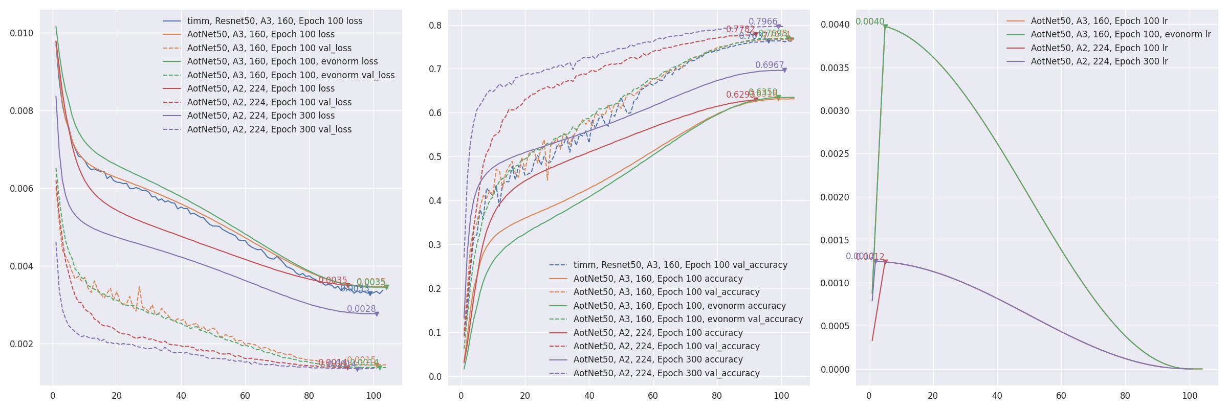
aotnet.AotNet50 的默认参数设置是一种典型的 ResNet50 架构,其中 Conv2D 使用 use_bias=False,且填充方式类似于 PyTorch。train_script.py 的默认参数配置类似于 ResNet 再出击:timm 中改进的训练流程 中的 A3 配置,即 batch_size=256, input_shape=(160, 160)。# 默认启用抗锯齿缩放,可通过设置 `--disable_antialias` 关闭。
CUDA_VISIBLE_DEVICES='0' TF_XLA_FLAGS="--tf_xla_auto_jit=2" python3 train_script.py --seed 0 -s aotnet50
# 使用输入尺寸 (224, 224) 进行评估。
# 抗锯齿的使用应与训练时一致。
CUDA_VISIBLE_DEVICES='1' python3 eval_script.py -m aotnet50_epoch_103_val_acc_0.7674.h5 -i 224 --central_crop 0.95
# >>>> 准确率 top1: 0.78466 top5: 0.94088
- 从断点恢复:通过设置
--restore_path 和 --initial_epoch 来实现,其他参数保持不变。restore_path 的优先级高于 model 和 additional_model_kwargs,同时会恢复 optimizer 和 loss。initial_epoch 主要用于学习率调度器。如果不确定停止的位置,可以查看 checkpoints/{save_name}_hist.json。import json
with open("checkpoints/aotnet50_hist.json", "r") as ff:
aa = json.load(ff)
len(aa['lr'])
# 41 ==> 已完成 41 个 epoch,因此 initial_epoch 为 41,从第 42 个 epoch 开始继续训练。
CUDA_VISIBLE_DEVICES='0' TF_XLA_FLAGS="--tf_xla_auto_jit=2" python3 train_script.py --seed 0 -r checkpoints/aotnet50_latest.h5 -I 41
# >>>> 从模型:checkpoints/aotnet50_latest.h5 恢复
# 第 42/105 个 epoch
eval_script.py 用于评估模型的准确率。EfficientNetV2 自测 ImageNet 准确率 #19 展示了不同参数如何影响模型的准确率。# 评估预训练的内置模型
CUDA_VISIBLE_DEVICES='1' python3 eval_script.py -m regnet.RegNetZD8
# 评估预训练的 timm 模型
CUDA_VISIBLE_DEVICES='1' python3 eval_script.py -m timm.models.resmlp_12_224 --input_shape 224
# 评估特定的 h5 模型
CUDA_VISIBLE_DEVICES='1' python3 eval_script.py -m checkpoints/xxx.h5
# 评估特定的 tflite 模型
CUDA_VISIBLE_DEVICES='1' python3 eval_script.py -m xxx.tflite
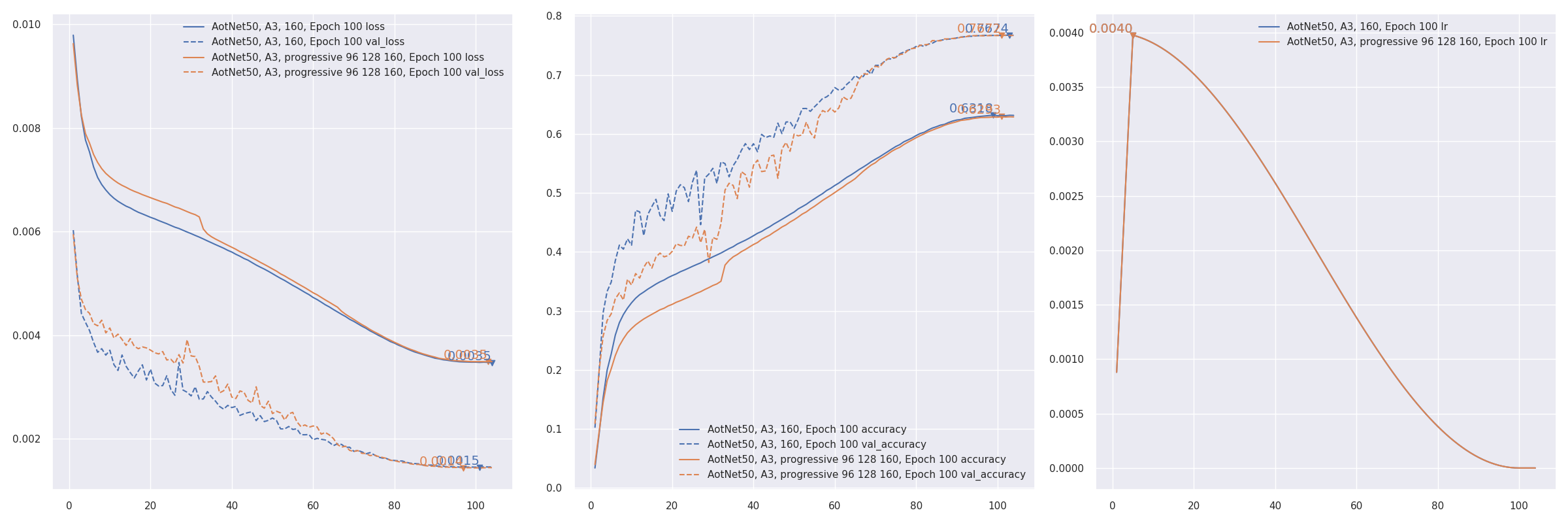
- 渐进式训练 参考 PDF 2104.00298 EfficientNetV2:更小的模型和更快的训练。AotNet50 A3 渐进式输入尺寸
96 128 160:CUDA_VISIBLE_DEVICES='1' TF_XLA_FLAGS="--tf_xla_auto_jit=2" python3 progressive_train_script.py \
--progressive_epochs 33 66 -1 \
--progressive_input_shapes 96 128 160 \
--progressive_magnitudes 2 4 6 \
-s aotnet50_progressive_3_lr_steps_100 --seed 0
- 使用
freeze_backbone 或 freeze_norm_layers 进行迁移学习:EfficientNetV2B0 在 cifar10 上进行迁移学习,测试冻结骨干网络 #55。
- CIFAR10 上的 Token Label 训练与测试 #57。目前效果未达预期。
Token label 是对 Github zihangJiang/TokenLabeling 的实现,相关论文为 PDF 2104.10858 所有 token 都重要:用于训练更好视觉 Transformer 的 Token Labeling。
COCO 训练与评估
目前仍在测试中。
COCO 提供了更详细的使用说明。
custom_dataset_script.py 可用于生成 json 格式的文件,该文件可作为 --data_name xxx.json 参数用于训练。详细用法请参见 自定义检测数据集。
coco_train_script.py 的默认参数为 EfficientDetD0,配置为 input_shape=(256, 256, 3), batch_size=64, mosaic_mix_prob=0.5, freeze_backbone_epochs=32, total_epochs=105。从技术上讲,任何 金字塔结构骨干 + EfficientDet / YOLOX 头部 / YOLOR 头部 + 无锚点 / yolor / efficientdet 锚点 的组合都是支持的。
目前支持四种类型的锚点,参数 anchors_mode 用于控制使用哪种锚点,取值为 ["efficientdet", "anchor_free", "yolor", "yolov8"]。对于 det_header 预设,默认为 None。
注意:YOLOV8 的边界框输出长度默认为 regression_len=64。通常其他检测模型为 4,而对于 yolov8 则是 reg_max=16 -> regression_len = 16 * 4 == 64。
| anchors_mode |
use_object_scores |
num_anchors |
anchor_scale |
aspect_ratios |
num_scales |
grid_zero_start |
| efficientdet |
False |
9 |
4 |
[1, 2, 0.5] |
3 |
False |
| anchor_free |
True |
1 |
1 |
[1] |
1 |
True |
| yolor |
True |
3 |
None |
预设 |
None |
offset=0.5 |
| yolov8 |
False |
1 |
1 |
[1] |
1 |
False |
# 默认 EfficientDetD0
CUDA_VISIBLE_DEVICES='0' python3 coco_train_script.py
# 默认 EfficientDetD0 使用 input_shape 512、优化器 adamw、冻结骨干 16 轮、总共 50 + 5 轮
CUDA_VISIBLE_DEVICES='0' python3 coco_train_script.py -i 512 -p adamw --freeze_backbone_epochs 16 --lr_decay_steps 50

# EfficientNetV2B0 骨干 + EfficientDetD0 检测头部
CUDA_VISIBLE_DEVICES='0' python3 coco_train_script.py --backbone efficientnet.EfficientNetV2B0 --det_header efficientdet.EfficientDetD0
# ResNest50 骨干 + EfficientDetD0 头部,使用类似 yolox 的无锚点锚点
CUDA_VISIBLE_DEVICES='0' python3 coco_train_script.py --backbone resnest.ResNest50 --anchors_mode anchor_free
# UniformerSmall32 骨干 + EfficientDetD0 头部,使用 yolor 锚点
CUDA_VISIBLE_DEVICES='0' python3 coco_train_script.py --backbone uniformer.UniformerSmall32 --anchors_mode yolor

# 典型的 YOLOXS,使用无锚点锚点
CUDA_VISIBLE_DEVICES='0' python3 coco_train_script.py --det_header yolox.YOLOXS --freeze_backbone_epochs 0
# YOLOXS 使用 efficientdet 锚点
CUDA_VISIBLE_DEVICES='0' python3 coco_train_script.py --det_header yolox.YOLOXS --anchors_mode efficientdet --freeze_backbone_epochs 0
# CoAtNet0 骨干 + YOLOX 头部,使用 yolor 锚点
CUDA_VISIBLE_DEVICES='0' python3 coco_train_script.py --backbone coatnet.CoAtNet0 --det_header yolox.YOLOX --anchors_mode yolor

# 典型的 YOLOR_P6,使用 yolor 锚点
CUDA_VISIBLE_DEVICES='0' python3 coco_train_script.py --det_header yolor.YOLOR_P6 --freeze_backbone_epochs 0
# YOLOR_P6 使用无锚点锚点
CUDA_VISIBLE_DEVICES='0' python3 coco_train_script.py --det_header yolor.YOLOR_P6 --anchors_mode anchor_free --freeze_backbone_epochs 0
# ConvNeXtTiny 骨干 + YOLOR 头部,使用 efficientdet 锚点
CUDA_VISIBLE_DEVICES='0' python3 coco_train_script.py --backbone convnext.ConvNeXtTiny --det_header yolor.YOLOR --anchors_mode yolor
注:COCO 训练仍在测试中,参数和默认行为可能会发生变化。如果您愿意参与开发,请自行承担风险。
coco_eval_script.py 用于在 COCO 验证集上评估模型的 AP / AR。它依赖于 pip install pycocotools,该包不在项目依赖中。更多用法请参见 COCO 评估。
# EfficientDetD0 使用双线性插值,不启用抗锯齿
CUDA_VISIBLE_DEVICES='1' python3 coco_eval_script.py -m efficientdet.EfficientDetD0 --resize_method bilinear --disable_antialias
# >>>> [COCOEvalCallback] input_shape: (512, 512), pyramid_levels: [3, 7], anchors_mode: efficientdet

# YOLOX 使用 BGR 输入格式
CUDA_VISIBLE_DEVICES='1' python3 coco_eval_script.py -m yolox.YOLOXTiny --use_bgr_input --nms_method hard --nms_iou_or_sigma 0.65
# >>>> [COCOEvalCallback] input_shape: (416, 416), pyramid_levels: [3, 5], anchors_mode: anchor_free

# YOLOR / YOLOV7 使用 letterbox_pad 等技巧
CUDA_VISIBLE_DEVICES='1' python3 coco_eval_script.py -m yolor.YOLOR_CSP --nms_method hard --nms_iou_or_sigma 0.65 \
--nms_max_output_size 300 --nms_topk -1 --letterbox_pad 64 --input_shape 704
# >>>> [COCOEvalCallback] input_shape: (704, 704), pyramid_levels: [3, 5], anchors_mode: yolor

# 指定 h5 模型
CUDA_VISIBLE_DEVICES='1' python3 coco_eval_script.py -m checkpoints/yoloxtiny_yolor_anchor.h5
# >>>> [COCOEvalCallback] input_shape: (416, 416), pyramid_levels: [3, 5], anchors_mode: yolor
[实验性] 使用 PyTorch 后端进行训练
import os, sys, torch
os.environ["KECAM_BACKEND"] = "torch"

from keras_cv_attention_models.yolov8 import train, yolov8
from keras_cv_attention_models import efficientnet

global_device = torch.device("cuda:0") if torch.cuda.is_available() and int(os.environ.get("CUDA_VISIBLE_DEVICES", "0")) >= 0 else torch.device("cpu")
# 模型可训练参数:7,023,904,GFLOPs:8.1815G
bb = efficientnet.EfficientNetV2B0(input_shape=(3, 640, 640), num_classes=0)
model = yolov8.YOLOV8_N(backbone=bb, classifier_activation=None,pretrained=None).to(global_device)  # 注意:classifier_activation=None
# 模型 = yolov8.YOLOV8_N(input_shape=(3, None, None),classifier_activation=None,pretrained=None).to(global_device)
ema = train.train(model, dataset_path="coco.json", initial_epoch=0)
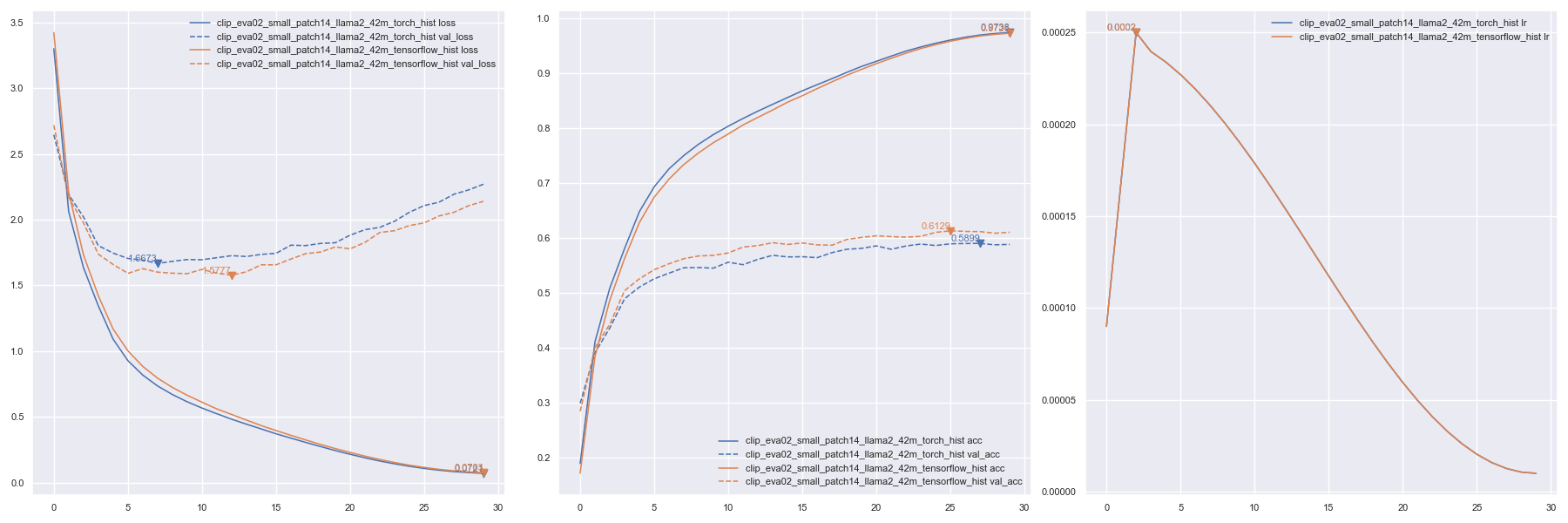
CLIP 训练与评估
- CLIP 提供了更详细的使用说明。
custom_dataset_script.py 可用于生成 tsv 或 json 格式的文件,该文件可作为 --data_name xxx.tsv 用于训练。详细用法请参见 自定义字幕数据集。- 使用
clip_train_script.py 在 COCO 字幕数据上训练 默认的 --data_path 是一个测试数据集 datasets/coco_dog_cat/captions.tsv。CUDA_VISIBLE_DEVICES=1 TF_XLA_FLAGS="--tf_xla_auto_jit=2" python clip_train_script.py -i 160 -b 128 \
--text_model_pretrained None --data_path coco_captions.tsv
通过设置 KECAM_BACKEND='torch' 使用 PyTorch 后端进行训练KECAM_BACKEND='torch' CUDA_VISIBLE_DEVICES=1 python clip_train_script.py -i 160 -b 128 \
--text_model_pretrained None --data_path coco_captions.tsv
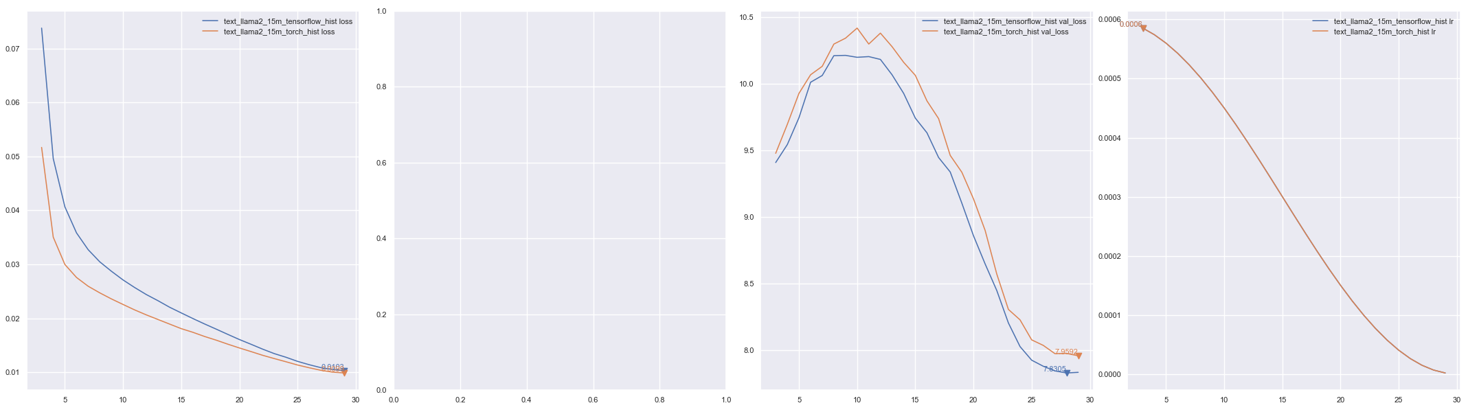
文本训练
- 目前这只是一个简单的实现,基于 Github karpathy/nanoGPT 修改而来。
- 使用
text_train_script.py 进行训练 由于数据集是随机采样的,需要指定 steps_per_epoch。CUDA_VISIBLE_DEVICES=1 TF_XLA_FLAGS="--tf_xla_auto_jit=2" python text_train_script.py -m LLaMA2_15M \
--steps_per_epoch 8000 --batch_size 8 --tokenizer SentencePieceTokenizer
通过设置 KECAM_BACKEND='torch' 使用 PyTorch 后端进行训练KECAM_BACKEND='torch' CUDA_VISIBLE_DEVICES=1 python text_train_script.py -m LLaMA2_15M \
--steps_per_epoch 8000 --batch_size 8 --tokenizer SentencePieceTokenizer
绘图from keras_cv_attention_models import plot_func
hists = ['checkpoints/text_llama2_15m_tensorflow_hist.json', 'checkpoints/text_llama2_15m_torch_hist.json']
plot_func.plot_hists(hists, addition_plots=['val_loss', 'lr'], skip_first=3)
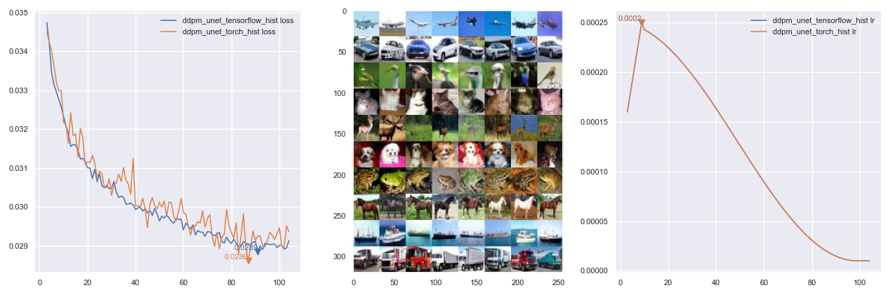
DDPM 训练
- Stable Diffusion 提供了更详细的使用说明。
- 注意:使用 PyTorch 后端效果更好,TensorFlow 后端在类似
--epochs 200 的训练日志中似乎更容易过拟合,且评估速度大约慢 5 倍。[???]
- 数据集 可以是一个仅包含图像的目录,用于仅使用图像的基础 DDPM 训练;也可以是一个按照 自定义识别数据集 创建的识别 JSON 文件,该文件将使用标签作为指令进行训练。
python custom_dataset_script.py --train_images cifar10/train/ --test_images cifar10/test/
# >>>> 总训练样本数:50000,总测试样本数:10000,类别数:10
# >>>> 已保存至:cifar10.json
- 使用
ddpm_train_script.py 在带有标签的 CIFAR10 数据集上训练 默认的 --data_path 是内置的 cifar10。# 将 --eval_interval 设置为 50,因为 TensorFlow 的评估速度较慢 [???]
TF_XLA_FLAGS="--tf_xla_auto_jit=2" CUDA_VISIBLE_DEVICES=1 python ddpm_train_script.py --eval_interval 50
通过设置 KECAM_BACKEND='torch' 使用 PyTorch 后端进行训练KECAM_BACKEND='torch' CUDA_VISIBLE_DEVICES=1 python ddpm_train_script.py
可视化
- Visualizing 用于可视化卷积神经网络的滤波器或注意力图得分。
- make_and_apply_gradcam_heatmap 用于 Grad-CAM 类激活可视化。
from keras_cv_attention_models import visualizing, test_images, resnest
mm = resnest.ResNest50()
img = test_images.dog()
superimposed_img, heatmap, preds = visualizing.make_and_apply_gradcam_heatmap(mm, img, layer_name="auto")
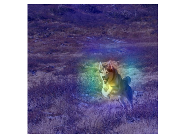
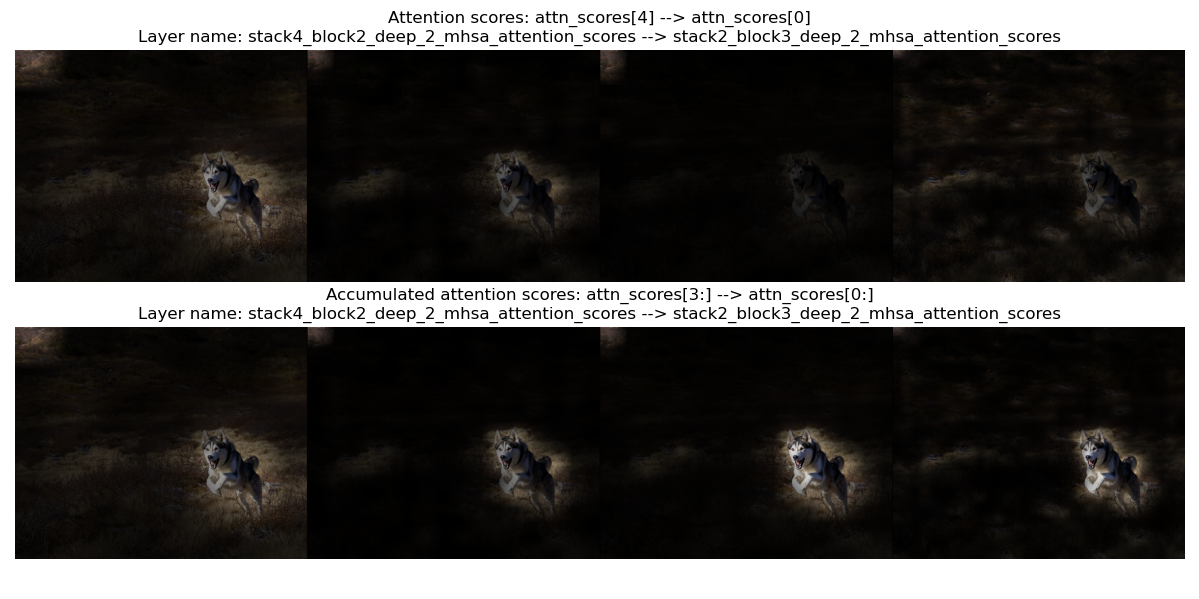
- plot_attention_score_maps 用于模型注意力得分图的可视化。
from keras_cv_attention_models import visualizing, test_images, botnet
img = test_images.dog()
_ = visualizing.plot_attention_score_maps(botnet.BotNetSE33T(), img)
TFLite 转换
- 目前
TFLite 不支持 tf.image.extract_patches 和 perm 长度大于 4 的 tf.transpose。某些操作在最新版本或 tf-nightly 版本中可能已支持,例如之前不支持的 gelu 和 groups>1 的 Conv2D 现在已经可以正常使用。如果遇到问题,可以尝试更新 TensorFlow 版本。
- 更多讨论请参见 将训练好的 Keras CV 注意力模型转换为 TFLite #17。一些速度测试结果可以在 如何加速量化模型的推理 #44 中找到。
- 使用最新版 TensorFlow 时,无需再使用诸如
model_surgery.convert_groups_conv2d_2_split_conv2d 和 model_surgery.convert_gelu_to_approximate 等函数。
- 不支持将
VOLO 和 HaloNet 模型转换为 TFLite 格式,因为这些模型需要更长的 tf.transpose perm。
- model_surgery.convert_dense_to_conv 会将所有具有 3D 或 4D 输入的
Dense 层转换为 Conv1D 或 Conv2D,因为当前 TFLite 的 xnnpack 尚不支持此类操作。from keras_cv_attention_models import beit, model_surgery, efficientformer, mobilevit
mm = efficientformer.EfficientFormerL1()
mm = model_surgery.convert_dense_to_conv(mm) # 将所有 Dense 层转换
converter = tf.lite.TFLiteConverter.from_keras_model(mm)
open(mm.name + ".tflite", "wb").write(converter.convert())
| 模型 |
Dense, use_xnnpack=false |
Conv, use_xnnpack=false |
Conv, use_xnnpack=true |
| MobileViT_S |
推理(平均)215371 us |
推理(平均)163836 us |
推理(平均)163817 us |
| EfficientFormerL1 |
推理(平均)126829 us |
推理(平均)107053 us |
推理(平均)107132 us |
- model_surgery.convert_extract_patches_to_conv 会将
tf.image.extract_patches 转换为等效的 Conv2D 实现:from keras_cv_attention_models import cotnet, model_surgery
from keras_cv_attention_models.imagenet import eval_func
mm = cotnet.CotNetSE50D()
mm = model_surgery.convert_groups_conv2d_2_split_conv2d(mm)
# mm = model_surgery.convert_gelu_to_approximate(mm) # 如果使用最新版 TFLite,则无需此步骤
mm = model_surgery.convert_extract_patches_to_conv(mm)
converter = tf.lite.TFLiteConverter.from_keras_model(mm)
open(mm.name + ".tflite", "wb").write(converter.convert())
test_inputs = np.random.uniform(size=[1, *mm.input_shape[1:]])
print(np.allclose(mm(test_inputs), eval_func.TFLiteModelInterf(mm.name + '.tflite')(test_inputs), atol=1e-7))
# True
- model_surgery.prepare_for_tflite 是上述功能的组合:
from keras_cv_attention_models import beit, model_surgery

mm = beit.BeitBasePatch16()
mm = model_surgery.prepare_for_tflite(mm)
converter = tf.lite.TFLiteConverter.from_keras_model(mm)
open(mm.name + ".tflite", "wb").write(converter.convert())
- 检测模型 包括
efficinetdet、yolox 和 yolor,可以直接转换为 TFLite 格式。如果需要将 DecodePredictions 也包含在 TFLite 模型中,则需将 DecodePredictions 的 use_static_output 设置为 True,因为 TFLite 要求输出形状更加静态。模型的输出形状将固定为 [batch, max_output_size, 6]。其中最后一维 6 表示 [bbox_top, bbox_left, bbox_bottom, bbox_right, label_index, confidence],有效预测是那些 confidence > 0 的结果。""" 初始化模型 """
from keras_cv_attention_models import efficientdet
model = efficientdet.EfficientDetD0(pretrained="coco")
""" 创建带有 DecodePredictions 的模型,并设置 `use_static_output=True` """
model.decode_predictions.use_static_output = True
# 如有需要,可调整 score_threshold 和 iou_or_sigma 等参数。
nn = model.decode_predictions(model.outputs[0], score_threshold=0.5)
bb = keras.models.Model(model.inputs[0], nn)
""" 转换为 TFLite """
converter = tf.lite.TFLiteConverter.from_keras_model(bb)
open(bb.name + ".tflite", "wb").write(converter.convert())
""" 推理测试 """
from keras_cv_attention_models.imagenet import eval_func
from keras_cv_attention_models import test_images
dd = eval_func.TFLiteModelInterf(bb.name + ".tflite")
imm = test_images.cat()
inputs = tf.expand_dims(tf.image.resize(imm, dd.input_shape[1:-1]), 0)
inputs = keras.applications.imagenet_utils.preprocess_input(inputs, mode='torch')
preds = dd(inputs)[0]
print(f"{preds.shape = }")
# preds.shape = (100, 6)
pred = preds[preds[:, -1] > 0]
bboxes, labels, confidences = pred[:, :4], pred[:, 4], pred[:, -1]
print(f"{bboxes = }, {labels = }, {confidences = }")
# bboxes = array([[0.22825494, 0.47238672, 0.816262 , 0.8700745 ]], dtype=float32),
# labels = array([16.], dtype=float32),
# confidences = array([0.8309707], dtype=float32)
""" 显示结果 """
from keras_cv_attention_models.coco import data
data.show_image_with_bboxes(imm, bboxes, labels, confidences, num_classes=90)
使用 PyTorch 作为后端
- 实验性 Keras PyTorch 后端。
- 设置环境变量
export KECAM_BACKEND='torch' 以启用此 PyTorch 后端。
- 目前支持大多数识别和检测模型,除了 hornet*gf / nfnets / volo。对于检测模型,在运行预测时使用
torchvision.ops.nms。
- 基本模型构建和预测。
- 如果可用,将加载与 TensorFlow 版本相同的
h5 权重。
- 注意:
input_shape 将自动适配图像数据格式。给定 input_shape=(224, 224, 3) 或 input_shape=(3, 224, 224),如果使用 channels_first 格式,两者都会被设置为 (3, 224, 224)。
- 注意:模型默认设置为
eval 模式。
os.environ['KECAM_BACKEND'] = 'torch'
from keras_cv_attention_models import res_mlp
mm = res_mlp.ResMLP12()
# >>>> 从 ~/.keras/models/resmlp12_imagenet.h5 加载预训练权重
print(f"{mm.input_shape = }")
# mm.input_shape = [None, 3, 224, 224]

import torch
print(f"{isinstance(mm, torch.nn.Module) = }")
# isinstance(mm, torch.nn.Module) = True

# 运行预测
from keras_cv_attention_models.test_images import cat
print(mm.decode_predictions(mm(mm.preprocess_input(cat())))[0])
# [('n02124075', 'Egyptian_cat', 0.9597896), ('n02123045', 'tabby', 0.012809471), ...]
- 导出典型的 PyTorch onnx / pth。
import torch
torch.onnx.export(mm, torch.randn(1, 3, *mm.input_shape[2:]), mm.name + ".onnx")

# 或者通过 export_onnx
mm.export_onnx()
# 导出的 onnx 文件:resmlp12.onnx

mm.export_pth()
# 导出的 pth 文件:resmlp12.pth
- 将权重保存为 h5 文件。该
h5 文件也可以在典型的 TensorFlow 后端模型中加载。目前仅支持权重,不包含模型结构。mm.save_weights("foo.h5")
- 使用 compile 和 fit 进行训练 注意:损失函数的参数应为
y_true, y_pred,而典型的 PyTorch 损失函数使用 y_pred, y_true。import torch
from keras_cv_attention_models.backend import models, layers
mm = models.Sequential([layers.Input([3, 32, 32]), layers.Conv2D(32, 3), layers.GlobalAveragePooling2D(), layers.Dense(10)])
if torch.cuda.is_available():
_ = mm.to("cuda")
xx = torch.rand([64, *mm.input_shape[1:]])
yy = torch.functional.F.one_hot(torch.randint(0, mm.output_shape[-1], size=[64]), mm.output_shape[-1]).float()
loss = lambda y_true, y_pred: (y_true - y_pred.float()).abs().mean()
# 将检查关键字参数以调用 `self.train_compile` 或 `torch.nn.Module.compile`
mm.compile(optimizer="AdamW", loss=loss, metrics='acc', grad_accumulate=4)
mm.fit(xx, yy, epochs=2, batch_size=4)
使用 keras core 作为后端
识别模型
AotNet
- Keras AotNet 只是一个类似于
ResNet / ResNetV2 的框架,通过设置如 attn_types 和 se_ratio 等参数来应用不同类型的注意力层。其工作方式类似于 timm 中的 byoanet / byobnet。
- 默认参数设置为典型的
ResNet 架构,其中 Conv2D 不使用偏置,填充方式类似于 PyTorch。from keras_cv_attention_models import aotnet
# 混合了 se、outlook、halo、mhsa 和 cot_attention,总参数量为 2100 万。
# 50 只是一个大于相对 `num_block` 的数字。
attn_types = [None, "outlook", ["bot", "halo"] * 50, "cot"],
se_ratio = [0.25, 0, 0, 0],
model = aotnet.AotNet50V2(attn_types=attn_types, se_ratio=se_ratio, stem_type="deep", strides=1)
model.summary()
BEiT
BEiTV2
| 模型 |
参数量 |
FLOPs |
输入 |
Top1 精度 |
T4 推理 |
| BeitV2BasePatch16 |
86.53M |
17.61G |
224 |
85.5 |
322.52 qps |
| - 21k_ft1k |
86.53M |
17.61G |
224 |
86.5 |
322.52 qps |
| BeitV2LargePatch16 |
304.43M |
61.68G |
224 |
87.3 |
105.734 qps |
| - 21k_ft1k |
304.43M |
61.68G |
224 |
88.4 |
105.734 qps |
BotNet
| 模型 |
参数量 |
FLOPs |
输入 |
Top1 精度 |
T4 推理 |
| BotNet50 |
21M |
5.42G |
224 |
|
746.454 qps |
| BotNet101 |
41M |
9.13G |
224 |
|
448.102 qps |
| BotNet152 |
56M |
12.84G |
224 |
|
316.671 qps |
| BotNet26T |
12.5M |
3.30G |
256 |
79.246 |
1188.84 qps |
| BotNextECA26T |
10.59M |
2.45G |
256 |
79.270 |
1038.19 qps |
| BotNetSE33T |
13.7M |
3.89G |
256 |
81.2 |
610.429 qps |
CAFormer
| 模型 |
参数量 |
FLOPs |
输入分辨率 |
Top1 准确率 |
T4 推理速度 |
| CAFormerS18 |
26M |
4.1G |
224 |
83.6 |
399.127 qps |
| - 384 |
26M |
13.4G |
384 |
85.0 |
181.993 qps |
| - 21k_ft1k |
26M |
4.1G |
224 |
84.1 |
399.127 qps |
| - 21k_ft1k, 384 |
26M |
13.4G |
384 |
85.4 |
181.993 qps |
| CAFormerS36 |
39M |
8.0G |
224 |
84.5 |
204.328 qps |
| - 384 |
39M |
26.0G |
384 |
85.7 |
102.04 qps |
| - 21k_ft1k |
39M |
8.0G |
224 |
85.8 |
204.328 qps |
| - 21k_ft1k, 384 |
39M |
26.0G |
384 |
86.9 |
102.04 qps |
| CAFormerM36 |
56M |
13.2G |
224 |
85.2 |
162.257 qps |
| - 384 |
56M |
42.0G |
384 |
86.2 |
65.6188 qps |
| - 21k_ft1k |
56M |
13.2G |
224 |
86.6 |
162.257 qps |
| - 21k_ft1k, 384 |
56M |
42.0G |
384 |
87.5 |
65.6188 qps |
| CAFormerB36 |
99M |
23.2G |
224 |
85.5 |
116.865 qps |
| - 384 |
99M |
72.2G |
384 |
86.4 |
50.0244 qps |
| - 21k_ft1k |
99M |
23.2G |
224 |
87.4 |
116.865 qps |
| - 21k_ft1k, 384 |
99M |
72.2G |
384 |
88.1 |
50.0244 qps |
CMT
CoaT
CoAtNet
| 模型 |
参数量 |
FLOPs |
输入尺寸 |
Top1准确率 |
T4推理速度 |
| CoAtNet0, 160, (105轮) |
23.3M |
2.09G |
160 |
80.48 |
584.059 qps |
| CoAtNet0, (305轮) |
23.8M |
4.22G |
224 |
82.79 |
400.333 qps |
| CoAtNet0 |
25M |
4.6G |
224 |
82.0 |
400.333 qps |
| - use_dw_strides=False |
25M |
4.2G |
224 |
81.6 |
461.197 qps |
| CoAtNet1 |
42M |
8.8G |
224 |
83.5 |
206.954 qps |
| - use_dw_strides=False |
42M |
8.4G |
224 |
83.3 |
228.938 qps |
| CoAtNet2 |
75M |
16.6G |
224 |
84.1 |
156.359 qps |
| - use_dw_strides=False |
75M |
15.7G |
224 |
84.1 |
165.846 qps |
| CoAtNet2, 21k_ft1k |
75M |
16.6G |
224 |
87.1 |
156.359 qps |
| CoAtNet3 |
168M |
34.7G |
224 |
84.5 |
95.0703 qps |
| CoAtNet3, 21k_ft1k |
168M |
34.7G |
224 |
87.6 |
95.0703 qps |
| CoAtNet3, 21k_ft1k |
168M |
203.1G |
512 |
87.9 |
95.0703 qps |
| CoAtNet4, 21k_ft1k |
275M |
360.9G |
512 |
88.1 |
74.6022 qps |
| CoAtNet4, 21k_ft1k, PT-RA-E150 |
275M |
360.9G |
512 |
88.56 |
74.6022 qps |
ConvNeXt
ConvNeXtV2
CoTNet
CSPNeXt
DaViT
| 模型 |
参数量 |
FLOPs |
输入大小 |
Top1 准确率 |
T4 推理速度 |
| DaViT_T |
28.36M |
4.56G |
224 |
82.8% |
224.563 qps |
| DaViT_S |
49.75M |
8.83G |
224 |
84.2% |
145.838 qps |
| DaViT_B |
87.95M |
15.55G |
224 |
84.6% |
114.527 qps |
| DaViT_L, 21k_ft1k |
196.8M |
103.2G |
384 |
87.5% |
34.7015 qps |
| DaViT_H, 1.5B |
348.9M |
327.3G |
512 |
90.2% |
12.363 qps |
| DaViT_G, 1.5B |
1.406B |
1.022T |
512 |
90.4% |
|
DiNAT
DINOv2
EdgeNeXt
EfficientFormer
EfficientFormerV2
EfficientNet
EfficientNetEdgeTPU
EfficientNetV2
EfficientViT_B
| 模型 |
参数量 |
FLOPs |
输入尺寸 |
Top1 准确率 |
T4 推理速度 |
| EfficientViT_B0 |
3.41M |
0.12G |
224 |
71.6 ? |
1581.76 qps |
| EfficientViT_B1 |
9.10M |
0.58G |
224 |
79.4 |
943.587 qps |
| - 256 |
9.10M |
0.78G |
256 |
79.9 |
840.844 qps |
| - 288 |
9.10M |
1.03G |
288 |
80.4 |
680.088 qps |
| EfficientViT_B2 |
24.33M |
1.68G |
224 |
82.1 |
583.295 qps |
| - 256 |
24.33M |
2.25G |
256 |
82.7 |
507.187 qps |
| - 288 |
24.33M |
2.92G |
288 |
83.1 |
419.93 qps |
| EfficientViT_B3 |
48.65M |
4.14G |
224 |
83.5 |
329.764 qps |
| - 256 |
48.65M |
5.51G |
256 |
83.8 |
288.605 qps |
| - 288 |
48.65M |
7.14G |
288 |
84.2 |
229.992 qps |
| EfficientViT_L1 |
52.65M |
5.28G |
224 |
84.48 |
503.068 qps |
| EfficientViT_L2 |
63.71M |
6.98G |
224 |
85.05 |
396.255 qps |
| - 384 |
63.71M |
20.7G |
384 |
85.98 |
207.322 qps |
| EfficientViT_L3 |
246.0M |
27.6G |
224 |
85.814 |
174.926 qps |
| - 384 |
246.0M |
81.6G |
384 |
86.408 |
86.895 qps |
EfficientViT_M
EVA
EVA02
FasterNet
FasterViT
FastViT
| 模型 |
参数量 |
FLOPs |
输入分辨率 |
Top1 准确率 |
T4 推理速度 |
| FastViT_T8 |
4.03M |
0.65G |
256 |
76.2 |
1020.29 qps |
| - 蒸馏版 |
4.03M |
0.65G |
256 |
77.2 |
1020.29 qps |
| - deploy=True |
3.99M |
0.64G |
256 |
76.2 |
1323.14 qps |
| FastViT_T12 |
7.55M |
1.34G |
256 |
79.3 |
734.867 qps |
| - 蒸馏版 |
7.55M |
1.34G |
256 |
80.3 |
734.867 qps |
| - deploy=True |
7.50M |
1.33G |
256 |
79.3 |
956.332 qps |
| FastViT_S12 |
9.47M |
1.74G |
256 |
79.9 |
666.669 qps |
| - 蒸馏版 |
9.47M |
1.74G |
256 |
81.1 |
666.669 qps |
| - deploy=True |
9.42M |
1.74G |
256 |
79.9 |
881.429 qps |
| FastViT_SA12 |
11.58M |
1.88G |
256 |
80.9 |
656.95 qps |
| - 蒸馏版 |
11.58M |
1.88G |
256 |
81.9 |
656.95 qps |
| - deploy=True |
11.54M |
1.88G |
256 |
80.9 |
833.011 qps |
| FastViT_SA24 |
21.55M |
3.66G |
256 |
82.7 |
371.84 qps |
| - 蒸馏版 |
21.55M |
3.66G |
256 |
83.4 |
371.84 qps |
| - deploy=True |
21.49M |
3.66G |
256 |
82.7 |
444.055 qps |
| FastViT_SA36 |
31.53M |
5.44G |
256 |
83.6 |
267.986 qps |
| - 蒸馏版 |
31.53M |
5.44G |
256 |
84.2 |
267.986 qps |
| - deploy=True |
31.44M |
5.43G |
256 |
83.6 |
325.967 qps |
| FastViT_MA36 |
44.07M |
7.64G |
256 |
83.9 |
211.928 qps |
| - 蒸馏版 |
44.07M |
7.64G |
256 |
84.6 |
211.928 qps |
| - deploy=True |
43.96M |
7.63G |
256 |
83.9 |
274.559 qps |
FBNetV3
| 模型 |
参数量 |
FLOPs |
输入分辨率 |
Top1 准确率 |
T4 推理速度 |
| FBNetV3B |
5.57M |
539.82M |
256 |
79.15 |
713.882 qps |
| FBNetV3D |
10.31M |
665.02M |
256 |
79.68 |
635.963 qps |
| FBNetV3G |
16.62M |
1379.30M |
256 |
82.05 |
478.835 qps |
FlexiViT
GCViT
GhostNet
| 模型 |
参数量 |
FLOPs |
输入尺寸 |
Top1 准确率 |
T4 推理速度 |
| GhostNet_050 |
2.59M |
42.6M |
224 |
66.88 |
1272.25 qps |
| GhostNet_100 |
5.18M |
141.7M |
224 |
74.16 |
1167.4 qps |
| GhostNet_130 |
7.36M |
227.7M |
224 |
75.79 |
1024.49 qps |
| - ssld |
7.36M |
227.7M |
224 |
79.38 |
1024.49 qps |
GhostNetV2
GMLP
| 模型 |
参数量 |
FLOPs |
输入尺寸 |
Top1 准确率 |
T4 推理速度 |
| GMLPTiny16 |
6M |
1.35G |
224 |
72.3 |
234.187 qps |
| GMLPS16 |
20M |
4.44G |
224 |
79.6 |
138.363 qps |
| GMLPB16 |
73M |
15.82G |
224 |
81.6 |
77.816 qps |
GPViT
| 模型 |
参数量 |
FLOPs |
输入尺寸 |
Top1 准确率 |
T4 推理速度 |
| GPViT_L1 |
9.59M |
6.15G |
224 |
80.5 |
210.166 qps |
| GPViT_L2 |
24.2M |
15.74G |
224 |
83.4 |
139.656 qps |
| GPViT_L3 |
36.7M |
23.54G |
224 |
84.1 |
131.284 qps |
| GPViT_L4 |
75.5M |
48.29G |
224 |
84.3 |
94.1899 qps |
HaloNet
Hiera
HorNet
IFormer
| 模型 |
参数量 |
FLOPs |
输入大小 |
Top1 准确率 |
T4 推理速度 |
| IFormerSmall |
19.9M |
4.88G |
224 |
83.4 |
254.392 qps |
| - 384 |
20.9M |
16.29G |
384 |
84.6 |
128.98 qps |
| IFormerBase |
47.9M |
9.44G |
224 |
84.6 |
147.868 qps |
| - 384 |
48.9M |
30.86G |
384 |
85.7 |
77.8391 qps |
| IFormerLarge |
86.6M |
14.12G |
224 |
84.6 |
113.434 qps |
| - 384 |
87.7M |
45.74G |
384 |
85.8 |
60.0292 qps |
InceptionNeXt
LCNet
| 模型 |
参数量 |
FLOPs |
输入大小 |
Top1准确率 |
T4推理速度 |
| LCNet050 |
1.88M |
46.02M |
224 |
63.10 |
3107.89 qps |
| - ssld |
1.88M |
46.02M |
224 |
66.10 |
3107.89 qps |
| LCNet075 |
2.36M |
96.82M |
224 |
68.82 |
3083.55 qps |
| LCNet100 |
2.95M |
158.28M |
224 |
72.10 |
2752.6 qps |
| - ssld |
2.95M |
158.28M |
224 |
74.39 |
2752.6 qps |
| LCNet150 |
4.52M |
338.05M |
224 |
73.71 |
2250.69 qps |
| LCNet200 |
6.54M |
585.35M |
224 |
75.18 |
2028.31 qps |
| LCNet250 |
9.04M |
900.16M |
224 |
76.60 |
1686.7 qps |
| - ssld |
9.04M |
900.16M |
224 |
80.82 |
1686.7 qps |
LeViT
MaxViT
MetaTransFormer
MLP混合器
| 模型 |
参数量 |
FLOPs |
输入 |
Top1准确率 |
T4推理 |
| MLPMixerS32, JFT |
19.1M |
1.01G |
224 |
68.70 |
488.839 qps |
| MLPMixerS16, JFT |
18.5M |
3.79G |
224 |
73.83 |
451.962 qps |
| MLPMixerB32, JFT |
60.3M |
3.25G |
224 |
75.53 |
247.629 qps |
| - sam |
60.3M |
3.25G |
224 |
72.47 |
247.629 qps |
| MLPMixerB16 |
59.9M |
12.64G |
224 |
76.44 |
207.423 qps |
| - 21k_ft1k |
59.9M |
12.64G |
224 |
80.64 |
207.423 qps |
| - sam |
59.9M |
12.64G |
224 |
77.36 |
207.423 qps |
| - JFT |
59.9M |
12.64G |
224 |
80.00 |
207.423 qps |
| MLPMixerL32, JFT |
206.9M |
11.30G |
224 |
80.67 |
95.1865 qps |
| MLPMixerL16 |
208.2M |
44.66G |
224 |
71.76 |
77.9928 qps |
| - 21k_ft1k |
208.2M |
44.66G |
224 |
82.89 |
77.9928 qps |
| - JFT |
208.2M |
44.66G |
224 |
84.82 |
77.9928 qps |
| - 448 |
208.2M |
178.54G |
448 |
83.91 |
|
| - 448, JFT |
208.2M |
178.54G |
448 |
86.78 |
|
| MLPMixerH14, JFT |
432.3M |
121.22G |
224 |
86.32 |
|
| - 448, JFT |
432.3M |
484.73G |
448 |
87.94 |
|
MobileNetV3
MobileViT
MobileViT_V2
MogaNet
NAT
| 模型 |
参数量 |
FLOPs |
输入分辨率 |
Top1准确率 |
T4推理速度 |
| NAT_Mini |
20.0M |
2.73G |
224 |
81.8 |
85.2324 qps |
| NAT_Tiny |
27.9M |
4.34G |
224 |
83.2 |
62.6147 qps |
| NAT_Small |
50.7M |
7.84G |
224 |
83.7 |
41.1545 qps |
| NAT_Base |
89.8M |
13.76G |
224 |
84.3 |
30.8989 qps |
NFNets
PVT_V2
| 模型 |
参数量 |
FLOPs |
输入尺寸 |
Top1 准确率 |
T4 推理速度 |
| PVT_V2B0 |
3.7M |
580.3M |
224 |
70.5 |
561.593 qps |
| PVT_V2B1 |
14.0M |
2.14G |
224 |
78.7 |
392.408 qps |
| PVT_V2B2 |
25.4M |
4.07G |
224 |
82.0 |
210.476 qps |
| PVT_V2B2_linear |
22.6M |
3.94G |
224 |
82.1 |
226.791 qps |
| PVT_V2B3 |
45.2M |
6.96G |
224 |
83.1 |
135.51 qps |
| PVT_V2B4 |
62.6M |
10.19G |
224 |
83.6 |
97.666 qps |
| PVT_V2B5 |
82.0M |
11.81G |
224 |
83.8 |
81.4798 qps |
RegNetY
| 模型 |
参数量 |
FLOPs |
输入尺寸 |
Top1 准确率 |
T4 推理速度 |
| RegNetY040 |
20.65M |
3.98G |
224 |
82.3 |
749.277 qps |
| RegNetY064 |
30.58M |
6.36G |
224 |
83.0 |
436.946 qps |
| RegNetY080 |
39.18M |
7.97G |
224 |
83.17 |
513.43 qps |
| RegNetY160 |
83.59M |
15.92G |
224 |
82.0 |
338.046 qps |
| RegNetY320 |
145.05M |
32.29G |
224 |
82.5 |
188.508 qps |
RegNetZ
RepViT
| 模型 |
参数量 |
FLOPs |
输入尺寸 |
Top1 准确率 |
T4 推理速度 |
| RepViT_M09, 蒸馏 |
5.10M |
0.82G |
224 |
79.1 |
|
| - deploy=True |
5.07M |
0.82G |
224 |
79.1 |
966.72 qps |
| RepViT_M10, 蒸馏 |
6.85M |
1.12G |
224 |
80.3 |
1157.8 qps |
| - deploy=True |
6.81M |
1.12G |
224 |
80.3 |
|
| RepViT_M11, 蒸馏 |
8.29M |
1.35G |
224 |
81.2 |
846.682 qps |
| - deploy=True |
8.24M |
1.35G |
224 |
81.2 |
1027.5 qps |
| RepViT_M15, 蒸馏 |
14.13M |
2.30G |
224 |
82.5 |
|
| - deploy=True |
14.05M |
2.30G |
224 |
82.5 |
|
| RepViT_M23, 蒸馏 |
23.01M |
4.55G |
224 |
83.7 |
|
| - deploy=True |
22.93M |
4.55G |
224 |
83.7 |
|
ResMLP
| 模型 |
参数量 |
FLOPs |
输入尺寸 |
Top1 准确率 |
T4 推理速度 |
| ResMLP12 |
15M |
3.02G |
224 |
77.8 |
928.402 qps |
| ResMLP24 |
30M |
5.98G |
224 |
80.8 |
420.709 qps |
| ResMLP36 |
116M |
8.94G |
224 |
81.1 |
309.513 qps |
| ResMLP_B24 |
129M |
100.39G |
224 |
83.6 |
78.3015 qps |
| - 21k_ft1k |
129M |
100.39G |
224 |
84.4 |
78.3015 qps |
ResNeSt
| 模型 |
参数量 |
FLOPs |
输入尺寸 |
Top1 准确率 |
T4 推理速度 |
| ResNest50 |
28M |
5.38G |
224 |
81.03 |
534.627 qps |
| ResNest101 |
49M |
13.33G |
256 |
82.83 |
257.074 qps |
| ResNest200 |
71M |
35.55G |
320 |
83.84 |
118.183 qps |
| ResNest269 |
111M |
77.42G |
416 |
84.54 |
61.167 qps |
ResNetD
| 模型 |
参数量 |
FLOPs |
输入尺寸 |
Top1 准确率 |
T4 推理速度 |
| ResNet50D |
25.58M |
4.33G |
224 |
80.530 |
930.214 qps |
| ResNet101D |
44.57M |
8.04G |
224 |
83.022 |
502.268 qps |
| ResNet152D |
60.21M |
11.75G |
224 |
83.680 |
353.279 qps |
| ResNet200D |
64.69M |
15.25G |
224 |
83.962 |
287.73 qps |
ResNetQ
| 模型 |
参数量 |
FLOPs |
输入尺寸 |
Top1 准确率 |
T4 推理速度 |
| ResNet51Q |
35.7M |
4.87G |
224 |
82.36 |
838.754 qps |
| ResNet61Q |
36.8M |
5.96G |
224 |
|
730.245 qps |
ResNeXt
SwinTransformerV2
TinyNet
| 模型 |
参数量 |
FLOPs |
输入大小 |
Top1 准确率 |
T4 推理速度 |
| TinyNetE |
2.04M |
25.22M |
106 |
59.86 |
2152.36 qps |
| TinyNetD |
2.34M |
53.35M |
152 |
66.96 |
1905.56 qps |
| TinyNetC |
2.46M |
103.22M |
184 |
71.23 |
1353.44 qps |
| TinyNetB |
3.73M |
206.28M |
188 |
74.98 |
1196.06 qps |
| TinyNetA |
6.19M |
343.74M |
192 |
77.65 |
981.976 qps |
TinyViT
UniFormer
VanillaNet
| 模型 |
参数量 |
FLOPs |
输入尺寸 |
Top1 准确率 |
T4 推理速度 |
| VanillaNet5 |
22.33M |
8.46G |
224 |
72.49 |
598.964 qps |
| - deploy=True |
15.52M |
5.17G |
224 |
72.49 |
798.199 qps |
| VanillaNet6 |
56.12M |
10.11G |
224 |
76.36 |
465.031 qps |
| - deploy=True |
32.51M |
6.00G |
224 |
76.36 |
655.944 qps |
| VanillaNet7 |
56.67M |
11.84G |
224 |
77.98 |
375.479 qps |
| - deploy=True |
32.80M |
6.90G |
224 |
77.98 |
527.723 qps |
| VanillaNet8 |
65.18M |
13.50G |
224 |
79.13 |
341.157 qps |
| - deploy=True |
37.10M |
7.75G |
224 |
79.13 |
479.328 qps |
| VanillaNet9 |
73.68M |
15.17G |
224 |
79.87 |
312.815 qps |
| - deploy=True |
41.40M |
8.59G |
224 |
79.87 |
443.464 qps |
| VanillaNet10 |
82.19M |
16.83G |
224 |
80.57 |
277.871 qps |
| - deploy=True |
45.69M |
9.43G |
224 |
80.57 |
408.082 qps |
| VanillaNet11 |
90.69M |
18.49G |
224 |
81.08 |
267.026 qps |
| - deploy=True |
50.00M |
10.27G |
224 |
81.08 |
377.239 qps |
| VanillaNet12 |
99.20M |
20.16G |
224 |
81.55 |
229.987 qps |
| - deploy=True |
54.29M |
11.11G |
224 |
81.55 |
358.076 qps |
| VanillaNet13 |
107.7M |
21.82G |
224 |
82.05 |
218.256 qps |
| - deploy=True |
58.59M |
11.96G |
224 |
82.05 |
334.244 qps |
ViT-5
VOLO
| 模型 |
参数量 |
FLOPs |
输入尺寸 |
Top1 准确率 |
T4 推理速度 |
| VOLO_d1 |
27M |
4.82G |
224 |
84.2 |
|
| - 384 |
27M |
14.22G |
384 |
85.2 |
|
| VOLO_d2 |
59M |
9.78G |
224 |
85.2 |
|
| - 384 |
59M |
28.84G |
384 |
86.0 |
|
| VOLO_d3 |
86M |
13.80G |
224 |
85.4 |
|
| - 448 |
86M |
55.50G |
448 |
86.3 |
|
| VOLO_d4 |
193M |
29.39G |
224 |
85.7 |
|
| - 448 |
193M |
117.81G |
448 |
86.8 |
|
| VOLO_d5 |
296M |
53.34G |
224 |
86.1 |
|
| - 448 |
296M |
213.72G |
448 |
87.0 |
|
| - 512 |
296M |
279.36G |
512 |
87.1 |
|
WaveMLP
| 模型 |
参数量 |
FLOPs |
输入大小 |
Top1 准确率 |
T4 推理速度 |
| WaveMLP_T |
17M |
2.47G |
224 |
80.9 |
523.4 qps |
| WaveMLP_S |
30M |
4.55G |
224 |
82.9 |
203.445 qps |
| WaveMLP_M |
44M |
7.92G |
224 |
83.3 |
147.155 qps |
| WaveMLP_B |
63M |
10.26G |
224 |
83.6 |
|
检测模型
EfficientDet
YOLO_NAS
YOLOR
| 模型 |
参数量 |
FLOPs |
输入大小 |
COCO 验证集 AP |
测试集 AP |
T4 推理速度 |
| YOLOR_CSP |
52.9M |
60.25G |
640 |
50.0 |
52.8 |
118.746 qps |
| YOLOR_CSPX |
99.8M |
111.11G |
640 |
51.5 |
54.8 |
67.9444 qps |
| YOLOR_P6 |
37.3M |
162.87G |
1280 |
52.5 |
55.7 |
49.3128 qps |
| YOLOR_W6 |
79.9M |
226.67G |
1280 |
53.6 ? |
56.9 |
40.2355 qps |
| YOLOR_E6 |
115.9M |
341.62G |
1280 |
50.3 ? |
57.6 |
21.5719 qps |
| YOLOR_D6 |
151.8M |
467.88G |
1280 |
50.8 ? |
58.2 |
16.6061 qps |
YOLOV7
| 模型 |
参数量 |
FLOPs |
输入大小 |
COCO 验证集 AP |
测试集 AP |
T4 推理速度 |
| YOLOV7_Tiny |
6.23M |
2.90G |
416 |
33.3 |
|
845.903 qps |
| YOLOV7_CSP |
37.67M |
53.0G |
640 |
51.4 |
|
137.441 qps |
| YOLOV7_X |
71.41M |
95.0G |
640 |
53.1 |
|
82.0534 qps |
| YOLOV7_W6 |
70.49M |
180.1G |
1280 |
54.9 |
|
49.9841 qps |
| YOLOV7_E6 |
97.33M |
257.6G |
1280 |
56.0 |
|
31.3852 qps |
| YOLOV7_D6 |
133.9M |
351.4G |
1280 |
56.6 |
|
26.1346 qps |
| YOLOV7_E6E |
151.9M |
421.7G |
1280 |
56.8 |
|
20.1331 qps |
YOLOV8
| 模型 |
参数量 |
FLOPs |
输入大小 |
COCO 验证集 AP |
测试集 AP |
T4 推理速度 |
| YOLOV8_N |
3.16M |
4.39G |
640 |
37.3 |
|
614.042 qps |
| YOLOV8_S |
11.17M |
14.33G |
640 |
44.9 |
|
349.528 qps |
| YOLOV8_M |
25.90M |
39.52G |
640 |
50.2 |
|
160.212 qps |
| YOLOV8_L |
43.69M |
82.65G |
640 |
52.9 |
|
104.452 qps |
| YOLOV8_X |
68.23M |
129.0G |
640 |
53.9 |
|
66.0428 qps |
| YOLOV8_X6 |
97.42M |
522.6G |
1280 |
56.7 ? |
|
17.4368 qps |
YOLOX
| 模型 |
参数量 |
FLOPs |
输入大小 |
COCO 验证集 AP |
测试集 AP |
T4 推理速度 |
| YOLOXNano |
0.91M |
0.53G |
416 |
25.8 |
|
930.57 qps |
| YOLOXTiny |
5.06M |
3.22G |
416 |
32.8 |
|
745.2 qps |
| YOLOXS |
9.0M |
13.39G |
640 |
40.5 |
40.5 |
380.38 qps |
| YOLOXM |
25.3M |
36.84G |
640 |
46.9 |
47.2 |
181.084 qps |
| YOLOXL |
54.2M |
77.76G |
640 |
49.7 |
50.1 |
111.517 qps |
| YOLOXX |
99.1M |
140.87G |
640 |
51.5 |
51.5 |
62.3189 qps |
语言模型
GPT2
LLaMA2
Stable Diffusion
| 模型 |
参数量 |
FLOPs |
输入 |
下载 |
| ViTTextLargePatch14 |
123.1M |
6.67G |
[None, 77] |
vit_text_large_patch14_clip.h5 |
| 编码器 |
34.16M |
559.6G |
[None, 512, 512, 3] |
encoder_v1_5.h5 |
| UNet |
859.5M |
404.4G |
[None, 64, 64, 4] |
unet_v1_5.h5 |
| 解码器 |
49.49M |
1259.5G |
[None, 64, 64, 4] |
decoder_v1_5.h5 |
分割模型
YOLOV8 分割
Segment Anything
许可证
引用
- BibTeX
@misc{leondgarse,
  author = {Leondgarse},
  title = {Keras CV 注意力模型},
  year = {2022},
  publisher = {GitHub},
  journal = {GitHub 仓库},
  doi = {10.5281/zenodo.6506947},
  howpublished = {\url{https://github.com/leondgarse/keras_cv_attention_models}}
}
- 最新 DOI:

Keras CV Attention Models 快速上手指南
keras_cv_attention_models (简称 kecam) 是一个集成了大量最新计算机视觉模型(如 ConvNeXt, Swin Transformer, YOLOv8, MobileViT 等)的 Keras 工具库,支持图像分类、目标检测、分割等任务。
1. 环境准备
系统要求
前置依赖
确保已安装以下基础科学计算库(若未安装):
pip install numpy pandas matplotlib
2. 安装步骤
推荐使用国内镜像源加速安装。
方式一:通过 PyPI 安装(推荐)
# 使用阿里云镜像源
pip install -U kecam -i https://mirrors.aliyun.com/pypi/simple/

# 或者使用完整包名
pip install -U keras-cv-attention-models -i https://mirrors.aliyun.com/pypi/simple/
方式二:从 GitHub 源码安装(获取最新功能)
pip install -U git+https://github.com/leondgarse/keras_cv_attention_models -i https://mirrors.aliyun.com/pypi/simple/
提示: 安装包 kecam 不强制绑定后端,请确保在安装前已自行安装好 TensorFlow 或 PyTorch。
3. 基本使用
3.1 图像分类(最简示例)
加载预训练模型并进行预测。库内置了 preprocess_input 和 decode_predictions 方便使用。
import tensorflow as tf
from keras_cv_attention_models import coatnet
from keras_cv_attention_models.test_images import cat

# 1. 加载预训练模型 (自动下载权重)
# 支持众多模型,如: convnext, swin_transformer_v2, mobilevit 等
mm = coatnet.CoAtNet0(pretrained="imagenet")

# 2. 准备图片并预处理
img = cat() # 加载测试图片
inputs = mm.preprocess_input(img)

# 3. 推理预测
preds = mm(tf.expand_dims(inputs, 0))

# 4. 解码结果
results = mm.decode_predictions(preds)
print(results[0])
# 输出示例: [('n02124075', 'Egyptian_cat', 0.9999875), ...]
3.2 自定义输出类别数
如果需要迁移学习,可以指定 num_classes。若类别数与预训练权重(通常为 1000)不一致,库会自动跳过顶层全连接层的权重加载。
from keras_cv_attention_models import swin_transformer_v2

# 设置为 64 类,顶层权重将不会加载,需重新训练该层
mm = swin_transformer_v2.SwinTransformerV2Tiny_window8(num_classes=64)
print(mm.summary())
3.3 提取特征(去除顶层)
设置 num_classes=0 可移除全局平均池化和全连接层,直接输出特征图。
from keras_cv_attention_models import resnest

# 输出形状将为 (None, H, W, Channels),无分类头
mm = resnest.ResNest50(num_classes=0)
print(mm.output_shape)
# 示例输出: (None, 7, 7, 2048)
3.4 使用别名简化导入
可以使用 kecam 作为简短别名:
import kecam

# 加载目标检测模型示例
model = kecam.yolor.YOLOR_CSP(pretrained="coco")
imgs = kecam.test_images.dog_cat()
preds = model(model.preprocess_input(imgs))

# 解码检测结果 (bbox, labels, confidences)
bboxes, labels, scores = model.decode_predictions(preds)[0]
3.5 切换 PyTorch 后端 (可选)
如果希望使用 PyTorch 作为后端运行模型:
import os
os.environ['KECAM_BACKEND'] = 'torch'

from keras_cv_attention_models import caformer

# 此时将使用 PyTorch 加载模型
mm = caformer.CAFormerS18(pretrained="imagenet")
print(f"Backend is using: {type(mm)}")
