D-FINE
D-FINE 是一个高效实时的目标检测模型,专为提升 DETR(Detection Transformer)系列模型的定位精度而设计。它将传统边界框回归任务重新定义为“细粒度分布优化”(Fine-grained Distribution Refinement, FDR),通过更精细地建模预测坐标的概率分布,显著提升了小目标和模糊边缘的检测准确性。同时,D-FINE 引入了“全局最优定位自蒸馏”(GO-LSD)机制,在不增加推理开销和训练成本的前提下,进一步优化模型性能。在 COCO 数据集上,D-FINE 在速度与精度之间取得了优异平衡,达到当前实时目标检测的领先水平。该模型特别适合计算机视觉领域的研究人员和算法工程师使用,尤其适用于对检测精度和推理效率有较高要求的场景,如自动驾驶、视频监控等。普通用户可通过 Hugging Face Spaces 快速体验其效果,但深度使用建议具备一定的深度学习基础。
使用场景
某智能交通系统开发团队正在部署城市道路监控方案,需在复杂光照条件和高密度车流中实时检测车辆、行人及交通标志。团队原采用YOLO系列模型,但在实际测试中发现多项性能瓶颈。
没有 D-FINE 时
- 小目标漏检严重:交通标志(如限速牌)因尺寸小、纹理简单,在逆光或雨雾天气下常被忽略
- 复杂场景精度下降:早高峰时段车流密集区域,模型对遮挡车辆的定位误差率高达18%
- 推理延迟影响实时性:4K分辨率视频流处理延迟达200ms,无法满足100ms内的实时响应要求
- 边界定位模糊:对运动模糊的电动车检测框存在15%的偏移量
- 模型泛化能力弱:从白天训练集迁移到夜间部署场景时,mAP值下降9.2个百分点
使用 D-FINE 后
- 小目标检测率提升:通过细粒度分布优化,限速牌等微小目标的召回率提高至92.7%
- 复杂场景鲁棒性增强:GO-LSD机制使遮挡车辆的定位误差降低至5.3%,支持更密集的物体检测
- 保持实时性的同时提升精度:在相同硬件条件下,4K视频处理延迟稳定在85ms以内
- 边缘定位更精准:运动模糊场景下检测框偏移量控制在3%以内,显著提升轨迹预测准确性
- 跨场景适应性优化:夜间场景mAP仅下降2.1个百分点,通过分布细化机制实现更好的光照不变性
D-FINE通过重构DETRs的回归范式,在不增加计算成本的前提下,实现了复杂交通场景下更精准、更鲁棒的实时目标检测,为智能交通系统提供了可靠的技术支撑。
运行环境要求
- Linux
- macOS
需要 NVIDIA GPU,显卡型号 T4 或更高,显存 8GB+,CUDA 11.7+
未说明
快速开始
English | 简体中文 | 日本語 | English Blog | 中文博客
D-FINE: 将 DETR 的回归任务重新定义为细粒度分布精炼(Fine‑grained Distribution Refinement)


![]()

📄 这是论文的官方实现:
D-FINE: 将 DETR 的回归任务重新定义为细粒度分布精炼(Fine-grained Distribution Refinement)
彭彦松、李河北、吴培曦、张悦怡、孙晓燕、吴枫
中国科学技术大学
![]()
如果您喜欢 D-FINE,请给我们一个 ⭐!您的支持将激励我们持续改进!

D-FINE 是一种强大的实时目标检测器,它将 DETR 中的边界框回归任务重新定义为细粒度分布精炼(Fine-grained Distribution Refinement, FDR),并引入了全局最优定位自蒸馏(Global Optimal Localization Self-Distillation, GO-LSD),在不增加额外推理和训练开销的前提下实现了卓越的性能。
视频演示
我们在来自 YouTube 的复杂街景视频上使用 D-FINE 和 YOLO11 进行目标检测。尽管面临逆光、运动模糊和人群密集等挑战,D-FINE-X 成功检测到了几乎所有目标,包括背包、自行车和交通灯等细微的小物体。其置信度分数以及对模糊边缘的定位精度显著优于 YOLO11。
https://github.com/user-attachments/assets/e5933d8e-3c8a-400e-870b-4e452f5321d9
🚀 更新日志
- [2024.10.18] 发布 D-FINE 系列模型。
- [2024.10.25] 添加自定义数据集微调配置 (#7)。
- [2024.10.30] 更新 D-FINE-L (E25) 预训练模型,性能提升 2.0%。
- [2024.11.07] 发布 D-FINE-N,在 COCO 上达到 42.8% APval @ 472 FPST4!
模型库(Model Zoo)
COCO
| 模型 | 数据集 | APval | 参数量 | 延迟 | GFLOPs | 配置文件 | 检查点 | 日志 |
|---|---|---|---|---|---|---|---|---|
| D‑FINE‑N | COCO | 42.8 | 4M | 2.12ms | 7 | yml | 42.8 | url |
| D‑FINE‑S | COCO | 48.5 | 10M | 3.49ms | 25 | yml | 48.5 | url |
| D‑FINE‑M | COCO | 52.3 | 19M | 5.62ms | 57 | yml | 52.3 | url |
| D‑FINE‑L | COCO | 54.0 | 31M | 8.07ms | 91 | yml | 54.0 | url |
| D‑FINE‑X | COCO | 55.8 | 62M | 12.89ms | 202 | yml | 55.8 | url |
Objects365+COCO
| Model | Dataset | APval | #Params | Latency | GFLOPs | config | checkpoint | logs |
|---|---|---|---|---|---|---|---|---|
| D‑FINE‑S | Objects365+COCO | 50.7 | 10M | 3.49ms | 25 | yml | 50.7 | url |
| D‑FINE‑M | Objects365+COCO | 55.1 | 19M | 5.62ms | 57 | yml | 55.1 | url |
| D‑FINE‑L | Objects365+COCO | 57.3 | 31M | 8.07ms | 91 | yml | 57.3 | url |
| D‑FINE‑X | Objects365+COCO | 59.3 | 62M | 12.89ms | 202 | yml | 59.3 | url |
We highly recommend that you use the Objects365 pre-trained model for fine-tuning:
⚠️ Important: Please note that this is generally beneficial for complex scene understanding. If your categories are very simple, it might lead to overfitting and suboptimal performance.
🔥 Pretrained Models on Objects365 (Best generalization)
| Model | Dataset | APval | AP5000 | #Params | Latency | GFLOPs | config | checkpoint | logs |
|---|---|---|---|---|---|---|---|---|---|
| D‑FINE‑S | Objects365 | 31.0 | 30.5 | 10M | 3.49ms | 25 | yml | 30.5 | url |
| D‑FINE‑M | Objects365 | 38.6 | 37.4 | 19M | 5.62ms | 57 | yml | 37.4 | url |
| D‑FINE‑L | Objects365 | - | 40.6 | 31M | 8.07ms | 91 | yml | 40.6 | url |
| D‑FINE‑L (E25) | Objects365 | 44.7 | 42.6 | 31M | 8.07ms | 91 | yml | 42.6 | url |
| D‑FINE‑X | Objects365 | 49.5 | 46.5 | 62M | 12.89ms | 202 | yml | 46.5 | url |
- E25: Re-trained and extended the pretraining to 25 epochs.
- APval is evaluated on Objects365 full validation set.
- AP5000 is evaluated on the first 5000 samples of the Objects365 validation set.
Notes:
- APval is evaluated on MSCOCO val2017 dataset.
- Latency is evaluated on a single T4 GPU with $batch\_size = 1$, $fp16$, and $TensorRT==10.4.0$.
- Objects365+COCO means finetuned model on COCO using pretrained weights trained on Objects365.
Quick start
Setup
conda create -n dfine python=3.11.9
conda activate dfine
pip install -r requirements.txt
Data Preparation
COCO2017 Dataset
Download COCO2017 from OpenDataLab or COCO.
Modify paths in coco_detection.yml
train_dataloader:
    img_folder: /data/COCO2017/train2017/
    ann_file: /data/COCO2017/annotations/instances_train2017.json
val_dataloader:
    img_folder: /data/COCO2017/val2017/
    ann_file: /data/COCO2017/annotations/instances_val2017.json
Objects365 Dataset
Download Objects365 from OpenDataLab.
Set the Base Directory:
export BASE_DIR=/data/Objects365/data
- Extract and organize the downloaded files, resulting directory structure:
${BASE_DIR}/train
├── images
│   ├── v1
│   │   ├── patch0
│   │   │   ├── 000000000.jpg
│   │   │   ├── 000000001.jpg
│   │   │   └── ... (more images)
│   ├── v2
│   │   ├── patchx
│   │   │   ├── 000000000.jpg
│   │   │   ├── 000000001.jpg
│   │   │   └── ... (more images)
├── zhiyuan_objv2_train.json
${BASE_DIR}/val
├── images
│   ├── v1
│   │   ├── patch0
│   │   │   ├── 000000000.jpg
│   │   │   └── ... (more images)
│   ├── v2
│   │   ├── patchx
│   │   │   ├── 000000000.jpg
│   │   │   └── ... (more images)
├── zhiyuan_objv2_val.json
- Create a New Directory to Store Images from the Validation Set:
mkdir -p ${BASE_DIR}/train/images_from_val
- Copy the v1 and v2 folders from the val directory into the train/images_from_val directory
cp -r ${BASE_DIR}/val/images/v1 ${BASE_DIR}/train/images_from_val/
cp -r ${BASE_DIR}/val/images/v2 ${BASE_DIR}/train/images_from_val/
- Run remap_obj365.py to merge a subset of the validation set into the training set. Specifically, this script moves samples with indices between 5000 and 800000 from the validation set to the training set.
python tools/remap_obj365.py --base_dir ${BASE_DIR}
- Run the resize_obj365.py script to resize any images in the dataset where the maximum edge length exceeds 640 pixels. Use the updated JSON file generated in Step 5 to process the sample data. Ensure that you resize images in both the train and val datasets to maintain consistency.
python tools/resize_obj365.py --base_dir ${BASE_DIR}
Modify paths in obj365_detection.yml
train_dataloader:
    img_folder: /data/Objects365/data/train
    ann_file: /data/Objects365/data/train/new_zhiyuan_objv2_train_resized.json
val_dataloader:
    img_folder: /data/Objects365/data/val/
    ann_file: /data/Objects365/data/val/new_zhiyuan_objv2_val_resized.json
CrowdHuman
Download COCO format dataset here: url
Custom Dataset
To train on your custom dataset, you need to organize it in the COCO format. Follow the steps below to prepare your dataset:
Set
remap_mscoco_categorytoFalse:This prevents the automatic remapping of category IDs to match the MSCOCO categories.
remap_mscoco_category: FalseOrganize Images:
Structure your dataset directories as follows:
dataset/ ├── images/ │ ├── train/ │ │ ├── image1.jpg │ │ ├── image2.jpg │ │ └── ... │ ├── val/ │ │ ├── image1.jpg │ │ ├── image2.jpg │ │ └── ... └── annotations/ ├── instances_train.json ├── instances_val.json └── ...images/train/: Contains all training images.images/val/: Contains all validation images.annotations/: Contains COCO-formatted annotation files.
Convert Annotations to COCO Format:
If your annotations are not already in COCO format, you'll need to convert them. You can use the following Python script as a reference or utilize existing tools:
import json

def convert_to_coco(input_annotations, output_annotations):
    # Implement conversion logic here
    pass

if __name__ == "__main__":
    convert_to_coco('path/to/your_annotations.json', 'dataset/annotations/instances_train.json')
Update Configuration Files:
Modify your custom_detection.yml.
task: detection

evaluator:
  type: CocoEvaluator
  iou_types: ['bbox', ]

num_classes: 777 # your dataset classes
remap_mscoco_category: False

train_dataloader:
  type: DataLoader
  dataset:
    type: CocoDetection
    img_folder: /data/yourdataset/train
    ann_file: /data/yourdataset/train/train.json
    return_masks: False
    transforms:
      type: Compose
      ops: ~
  shuffle: True
  num_workers: 4
  drop_last: True
  collate_fn:
    type: BatchImageCollateFunction

val_dataloader:
  type: DataLoader
  dataset:
    type: CocoDetection
    img_folder: /data/yourdataset/val
    ann_file: /data/yourdataset/val/ann.json
    return_masks: False
    transforms:
      type: Compose
      ops: ~
  shuffle: False
  num_workers: 4
  drop_last: False
  collate_fn:
    type: BatchImageCollateFunction
Usage
COCO2017
- Set Model
export model=l # n s m l x
- Training
CUDA_VISIBLE_DEVICES=0,1,2,3 torchrun --master_port=7777 --nproc_per_node=4 train.py -c configs/dfine/dfine_hgnetv2_${model}_coco.yml --use-amp --seed=0
- Testing
CUDA_VISIBLE_DEVICES=0,1,2,3 torchrun --master_port=7777 --nproc_per_node=4 train.py -c configs/dfine/dfine_hgnetv2_${model}_coco.yml --test-only -r model.pth
- Tuning
CUDA_VISIBLE_DEVICES=0,1,2,3 torchrun --master_port=7777 --nproc_per_node=4 train.py -c configs/dfine/dfine_hgnetv2_${model}_coco.yml --use-amp --seed=0 -t model.pth
Objects365 to COCO2017
- Set Model
export model=l # n s m l x
- Training on Objects365
CUDA_VISIBLE_DEVICES=0,1,2,3 torchrun --master_port=7777 --nproc_per_node=4 train.py -c configs/dfine/objects365/dfine_hgnetv2_${model}_obj365.yml --use-amp --seed=0
- Tuning on COCO2017
CUDA_VISIBLE_DEVICES=0,1,2,3 torchrun --master_port=7777 --nproc_per_node=4 train.py -c configs/dfine/objects365/dfine_hgnetv2_${model}_obj2coco.yml --use-amp --seed=0 -t model.pth
- Testing
CUDA_VISIBLE_DEVICES=0,1,2,3 torchrun --master_port=7777 --nproc_per_node=4 train.py -c configs/dfine/dfine_hgnetv2_${model}_coco.yml --test-only -r model.pth
Custom Dataset
- Set Model
export model=l # n s m l x
- Training on Custom Dataset
CUDA_VISIBLE_DEVICES=0,1,2,3 torchrun --master_port=7777 --nproc_per_node=4 train.py -c configs/dfine/custom/dfine_hgnetv2_${model}_custom.yml --use-amp --seed=0
- Testing
CUDA_VISIBLE_DEVICES=0,1,2,3 torchrun --master_port=7777 --nproc_per_node=4 train.py -c configs/dfine/custom/dfine_hgnetv2_${model}_custom.yml --test-only -r model.pth
- Tuning on Custom Dataset
CUDA_VISIBLE_DEVICES=0,1,2,3 torchrun --master_port=7777 --nproc_per_node=4 train.py -c configs/dfine/custom/objects365/dfine_hgnetv2_${model}_obj2custom.yml --use-amp --seed=0 -t model.pth
- [Optional] Modify Class Mappings:
When using the Objects365 pre-trained weights to train on your custom dataset, the example assumes that your dataset only contains the classes 'Person' and 'Car'. For faster convergence, you can modify self.obj365_ids in src/solver/_solver.py as follows:
self.obj365_ids = [0, 5] # Person, Cars
You can replace these with any corresponding classes from your dataset. The list of Objects365 classes with their corresponding IDs: https://github.com/Peterande/D-FINE/blob/352a94ece291e26e1957df81277bef00fe88a8e3/src/solver/_solver.py#L330
New training command:
CUDA_VISIBLE_DEVICES=0,1,2,3 torchrun --master_port=7777 --nproc_per_node=4 train.py -c configs/dfine/custom/dfine_hgnetv2_${model}_custom.yml --use-amp --seed=0 -t model.pth
However, if you don't wish to modify the class mappings, the pre-trained Objects365 weights will still work without any changes. Modifying the class mappings is optional and can potentially accelerate convergence for specific tasks.
Customizing Batch Size
For example, if you want to double the total batch size when training D-FINE-L on COCO2017, here are the steps you should follow:
Modify your dataloader.yml to increase the
total_batch_size:train_dataloader: total_batch_size: 64 # Previously it was 32, now doubledModify your dfine_hgnetv2_l_coco.yml. Here’s how the key parameters should be adjusted:
optimizer:
type: AdamW
params:
    -
    params: '^(?=.*backbone)(?!.*norm|bn).*$'
    lr: 0.000025  # doubled, linear scaling law
    -
    params: '^(?=.*(?:encoder|decoder))(?=.*(?:norm|bn)).*$'
    weight_decay: 0.

lr: 0.0005  # doubled, linear scaling law
betas: [0.9, 0.999]
weight_decay: 0.0001  # need a grid search

ema:  # added EMA settings
    decay: 0.9998  # adjusted by 1 - (1 - decay) * 2
    warmups: 500  # halved

lr_warmup_scheduler:
    warmup_duration: 250  # halved
Customizing Input Size
If you'd like to train D-FINE-L on COCO2017 with an input size of 320x320, follow these steps:
Modify your dataloader.yml:
train_dataloader:
dataset:
    transforms:
        ops:
            - {type: Resize, size: [320, 320], }
collate_fn:
    base_size: 320
dataset:
    transforms:
        ops:
            - {type: Resize, size: [320, 320], }
Modify your dfine_hgnetv2.yml:
eval_spatial_size: [320, 320]
Tools
Deployment
- Setup
pip install onnx onnxsim
export model=l  # n s m l x
- Export onnx
python tools/deployment/export_onnx.py --check -c configs/dfine/dfine_hgnetv2_${model}_coco.yml -r model.pth
- Export tensorrt
trtexec --onnx="model.onnx" --saveEngine="model.engine" --fp16
Inference (Visualization)
- Setup
pip install -r tools/inference/requirements.txt
export model=l  # n s m l x
- Inference (onnxruntime / tensorrt / torch)
Inference on images and videos is now supported.
python tools/inference/onnx_inf.py --onnx model.onnx --input image.jpg  # video.mp4
python tools/inference/trt_inf.py --trt model.engine --input image.jpg
python tools/inference/torch_inf.py -c configs/dfine/dfine_hgnetv2_${model}_coco.yml -r model.pth --input image.jpg --device cuda:0
Benchmark
- Setup
pip install -r tools/benchmark/requirements.txt
export model=l  # n s m l x
- Model FLOPs, MACs, and Params
python tools/benchmark/get_info.py -c configs/dfine/dfine_hgnetv2_${model}_coco.yml
- TensorRT Latency
python tools/benchmark/trt_benchmark.py --COCO_dir path/to/COCO2017 --engine_dir model.engine
Fiftyone Visualization
- Setup
pip install fiftyone
export model=l  # n s m l x
- Voxel51 Fiftyone Visualization (fiftyone)
python tools/visualization/fiftyone_vis.py -c configs/dfine/dfine_hgnetv2_${model}_coco.yml -r model.pth
Others
- Auto Resume Training
bash reference/safe_training.sh
- Converting Model Weights
python reference/convert_weight.py model.pth
Figures and Visualizations
FDR and GO-LSD
- Overview of D-FINE with FDR. The probability distributions that act as a more fine- grained intermediate representation are iteratively refined by the decoder layers in a residual manner. Non-uniform weighting functions are applied to allow for finer localization.
- Overview of GO-LSD process. Localization knowledge from the final layer’s refined distributions is distilled into earlier layers through DDF loss with decoupled weighting strategies.
Distributions
Visualizations of FDR across detection scenarios with initial and refined bounding boxes, along with unweighted and weighted distributions.
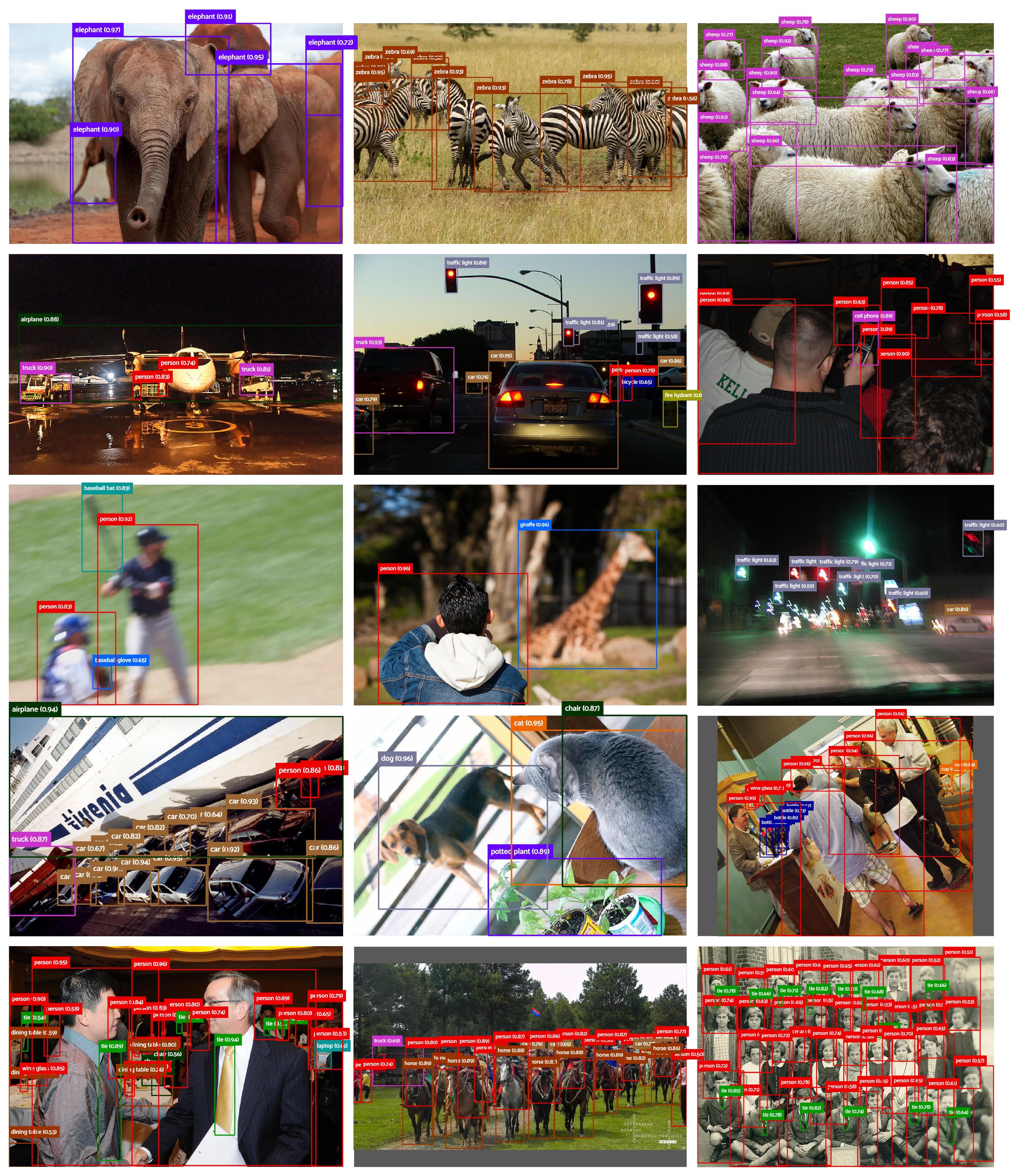
Hard Cases
The following visualization demonstrates D-FINE's predictions in various complex detection scenarios. These include cases with occlusion, low-light conditions, motion blur, depth of field effects, and densely populated scenes. Despite these challenges, D-FINE consistently produces accurate localization results.
Citation
If you use D-FINE or its methods in your work, please cite the following BibTeX entries:
bibtex
@misc{peng2024dfine,
      title={D-FINE: Redefine Regression Task in DETRs as Fine-grained Distribution Refinement},
      author={Yansong Peng and Hebei Li and Peixi Wu and Yueyi Zhang and Xiaoyan Sun and Feng Wu},
      year={2024},
      eprint={2410.13842},
      archivePrefix={arXiv},
      primaryClass={cs.CV}
}
Acknowledgement
Our work is built upon RT-DETR. Thanks to the inspirations from RT-DETR, GFocal, LD, and YOLOv9.
✨ Feel free to contribute and reach out if you have any questions! ✨
常见问题
相似工具推荐
stable-diffusion-webui
stable-diffusion-webui 是一个基于 Gradio 构建的网页版操作界面,旨在让用户能够轻松地在本地运行和使用强大的 Stable Diffusion 图像生成模型。它解决了原始模型依赖命令行、操作门槛高且功能分散的痛点,将复杂的 AI 绘图流程整合进一个直观易用的图形化平台。 无论是希望快速上手的普通创作者、需要精细控制画面细节的设计师,还是想要深入探索模型潜力的开发者与研究人员,都能从中获益。其核心亮点在于极高的功能丰富度:不仅支持文生图、图生图、局部重绘(Inpainting)和外绘(Outpainting)等基础模式,还独创了注意力机制调整、提示词矩阵、负向提示词以及“高清修复”等高级功能。此外,它内置了 GFPGAN 和 CodeFormer 等人脸修复工具,支持多种神经网络放大算法,并允许用户通过插件系统无限扩展能力。即使是显存有限的设备,stable-diffusion-webui 也提供了相应的优化选项,让高质量的 AI 艺术创作变得触手可及。
ComfyUI
ComfyUI 是一款功能强大且高度模块化的视觉 AI 引擎,专为设计和执行复杂的 Stable Diffusion 图像生成流程而打造。它摒弃了传统的代码编写模式,采用直观的节点式流程图界面,让用户通过连接不同的功能模块即可构建个性化的生成管线。 这一设计巧妙解决了高级 AI 绘图工作流配置复杂、灵活性不足的痛点。用户无需具备编程背景,也能自由组合模型、调整参数并实时预览效果,轻松实现从基础文生图到多步骤高清修复等各类复杂任务。ComfyUI 拥有极佳的兼容性,不仅支持 Windows、macOS 和 Linux 全平台,还广泛适配 NVIDIA、AMD、Intel 及苹果 Silicon 等多种硬件架构,并率先支持 SDXL、Flux、SD3 等前沿模型。 无论是希望深入探索算法潜力的研究人员和开发者,还是追求极致创作自由度的设计师与资深 AI 绘画爱好者,ComfyUI 都能提供强大的支持。其独特的模块化架构允许社区不断扩展新功能,使其成为当前最灵活、生态最丰富的开源扩散模型工具之一,帮助用户将创意高效转化为现实。
ML-For-Beginners
ML-For-Beginners 是由微软推出的一套系统化机器学习入门课程,旨在帮助零基础用户轻松掌握经典机器学习知识。这套课程将学习路径规划为 12 周,包含 26 节精炼课程和 52 道配套测验,内容涵盖从基础概念到实际应用的完整流程,有效解决了初学者面对庞大知识体系时无从下手、缺乏结构化指导的痛点。 无论是希望转型的开发者、需要补充算法背景的研究人员,还是对人工智能充满好奇的普通爱好者,都能从中受益。课程不仅提供了清晰的理论讲解,还强调动手实践,让用户在循序渐进中建立扎实的技能基础。其独特的亮点在于强大的多语言支持,通过自动化机制提供了包括简体中文在内的 50 多种语言版本,极大地降低了全球不同背景用户的学习门槛。此外,项目采用开源协作模式,社区活跃且内容持续更新,确保学习者能获取前沿且准确的技术资讯。如果你正寻找一条清晰、友好且专业的机器学习入门之路,ML-For-Beginners 将是理想的起点。
ragflow
RAGFlow 是一款领先的开源检索增强生成(RAG)引擎,旨在为大语言模型构建更精准、可靠的上下文层。它巧妙地将前沿的 RAG 技术与智能体(Agent)能力相结合,不仅支持从各类文档中高效提取知识,还能让模型基于这些知识进行逻辑推理和任务执行。 在大模型应用中,幻觉问题和知识滞后是常见痛点。RAGFlow 通过深度解析复杂文档结构(如表格、图表及混合排版),显著提升了信息检索的准确度,从而有效减少模型“胡编乱造”的现象,确保回答既有据可依又具备时效性。其内置的智能体机制更进一步,使系统不仅能回答问题,还能自主规划步骤解决复杂问题。 这款工具特别适合开发者、企业技术团队以及 AI 研究人员使用。无论是希望快速搭建私有知识库问答系统,还是致力于探索大模型在垂直领域落地的创新者,都能从中受益。RAGFlow 提供了可视化的工作流编排界面和灵活的 API 接口,既降低了非算法背景用户的上手门槛,也满足了专业开发者对系统深度定制的需求。作为基于 Apache 2.0 协议开源的项目,它正成为连接通用大模型与行业专有知识之间的重要桥梁。
PaddleOCR
PaddleOCR 是一款基于百度飞桨框架开发的高性能开源光学字符识别工具包。它的核心能力是将图片、PDF 等文档中的文字提取出来,转换成计算机可读取的结构化数据,让机器真正“看懂”图文内容。 面对海量纸质或电子文档,PaddleOCR 解决了人工录入效率低、数字化成本高的问题。尤其在人工智能领域,它扮演着连接图像与大型语言模型(LLM)的桥梁角色,能将视觉信息直接转化为文本输入,助力智能问答、文档分析等应用场景落地。 PaddleOCR 适合开发者、算法研究人员以及有文档自动化需求的普通用户。其技术优势十分明显:不仅支持全球 100 多种语言的识别,还能在 Windows、Linux、macOS 等多个系统上运行,并灵活适配 CPU、GPU、NPU 等各类硬件。作为一个轻量级且社区活跃的开源项目,PaddleOCR 既能满足快速集成的需求,也能支撑前沿的视觉语言研究,是处理文字识别任务的理想选择。
tesseract
Tesseract 是一款历史悠久且备受推崇的开源光学字符识别(OCR)引擎,最初由惠普实验室开发,后由 Google 维护,目前由全球社区共同贡献。它的核心功能是将图片中的文字转化为可编辑、可搜索的文本数据,有效解决了从扫描件、照片或 PDF 文档中提取文字信息的难题,是数字化归档和信息自动化的重要基础工具。 在技术层面,Tesseract 展现了强大的适应能力。从版本 4 开始,它引入了基于长短期记忆网络(LSTM)的神经网络 OCR 引擎,显著提升了行识别的准确率;同时,为了兼顾旧有需求,它依然支持传统的字符模式识别引擎。Tesseract 原生支持 UTF-8 编码,开箱即用即可识别超过 100 种语言,并兼容 PNG、JPEG、TIFF 等多种常见图像格式。输出方面,它灵活支持纯文本、hOCR、PDF、TSV 等多种格式,方便后续数据处理。 Tesseract 主要面向开发者、研究人员以及需要构建文档处理流程的企业用户。由于它本身是一个命令行工具和库(libtesseract),不包含图形用户界面(GUI),因此最适合具备一定编程能力的技术人员集成到自动化脚本或应用程序中